| The CALIS Procedure |
| Assessment of Fit |
In PROC CALIS, there are three main tools for assessing model fit:
residuals for the fitted means or covariances
overall model fit indices
squared multiple correlations and determination coefficients
This section contains a collection of formulas for these assessment tools. The following notation is used:
 for the total sample size
  for the total number of independent groups in analysis
  for the number of manifest variables
  for the number of parameters to estimate
  for the -vector of parameters,
  for the estimated parameters
  for the
  input covariance or correlation matrix
  for the -vector of sample means
  for the predicted covariance or correlation matrix
  for the predicted mean vector
  for indicating the modeling of the mean structures
  for the weight matrix
  for the minimized function value of the fitted model
  for the degrees of freedom of the fitted model
In multiple-group analyses, subscripts are used to distinguish independent groups or samples. For example, 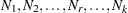 denote the sample sizes for groups. Similarly, notation such as
  ,
,  ,
,  ,
,  ,
,  ,
,  , and
, and  is used for multiple-group situations.
Residuals
Residuals indicate how well each entry or element in the mean or covariance matrix is fitted. Large residuals indicate bad fit.
PROC CALIS computes four types of residuals and writes them to the OUTSTAT= data set when requested.
raw residuals

for the covariance and mean residuals, respectively. The raw residuals are displayed whenever the PALL, PRINT, or RESIDUAL option is specified.
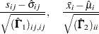
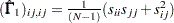
variance standardized residuals
for the covariance and mean residuals, respectively. The variance standardized residuals are displayed when you specify one of the following:
The variance standardized residuals are equal to those computed by the EQS 3 program (Bentler; 1995).
asymptotically standardized residuals
for the covariance and mean residuals, respectively; with

where
 is the
  estimated asymptotic covariance matrix of sample covariances,
  is the estimated asymptotic covariance matrix of sample means,
  is the
  Jacobian matrix
  ,
,  is the
  Jacobian matrix
  , and
, and  is the
  estimated covariance matrix of parameter estimates, all evaluated at the sample moments and estimated parameter values. See the next section for the definitions of and . Asymptotically standardized residuals are displayed when one of the following conditions is met:
 The PALL, the PRINT, or the RESIDUAL option is specified, and METHOD=ML, METHOD=GLS, or METHOD=WLS, and the expensive information and Jacobian matrices are computed for some other reason.
RESIDUAL= ASYSTAND is specified.
The asymptotically standardized residuals are equal to those computed by the LISREL 7 program (Jöreskog and Sörbom; 1988) except for the denominator in the definition of matrix
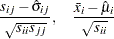
. normalized residuals
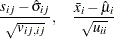
for the covariance and mean residuals, respectively; with
as the estimated asymptotic covariance matrix of sample covariances; and as the estimated asymptotic covariance matrix of sample means. Diagonal elements of
and are defined for the following methods: GLS:
 and
and 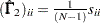
ML:
 and
and 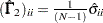
WLS:
 and
and
where
in the WLS method is the weight matrix for the second-order moments. Normalized residuals are displayed when one of the following conditions is met:
The PALL, PRINT, or RESIDUAL option is specified, and METHOD=ML, METHOD=GLS, or METHOD=WLS, and the expensive information and Jacobian matrices are not computed for some other reasons.
RESIDUAL=NORM is specified.
The normalized residuals are equal to those computed by the LISREL VI program (Jöreskog and Sörbom; 1985) except for the definition of the denominator in computing matrix
.
For estimation methods that are not "best" generalized least squares estimators (Browne; 1982, 1984), such as METHOD=NONE, METHOD=ULS, or METHOD=DWLS, the assumption of an asymptotic covariance matrix  of sample covariances does not seem to be appropriate. In this case, the normalized residuals should be replaced by the more relaxed variance standardized residuals. Computation of asymptotically standardized residuals requires computing the Jacobian and information matrices. This is computationally very expensive and is done only if the Jacobian matrix has to be computed for some other reasons—that is, if at least one of the following items is true:
The default, PRINT, or PALL displayed output is requested, and neither the NOMOD nor NOSTDERR option is specified.
Either the MODIFICATION (included in PALL), PCOVES, or STDERR (included in default, PRINT, and PALL output) option is requested or RESIDUAL=ASYSTAND is specified.
The LEVMAR or NEWRAP optimization technique is used.
An OUTMODEL= data set is specified without using the NOSTDERR option.
An OUTEST= data set is specified without using the NOSTDERR option.
Since normalized residuals use an overestimate of the asymptotic covariance matrix of residuals (the diagonals of and  ), the normalized residuals cannot be larger than the asymptotically standardized residuals (which use the diagonal of the form
  ).
).
Together with the residual matrices, the values of the average residual, the average off-diagonal residual, and the rank order of the largest values are displayed. The distributions of the normalized and standardized residuals are displayed also.
Overall Model Fit Indices
Instead of assessing the model fit by looking at a number of residuals of the fitted moments, an overall model fit index measures model fit by a single number. Although an overall model fit index is precise and easy to use, there are indeed many choices of overall fit indices. Unfortunately, researchers do not always have a consensus on the best set of indices to use in all occasions.
PROC CALIS produces a large number of overall model fit indices in the fit summary table. If you prefer to display only a subset of these fit indices, you can use the ONLIST(ONLY)= option of the FITINDEX statement to customize the fit summary table.
Fit indices are classified into three classes in the fit summary table of PROC CALIS:
absolute or standalone Indices
parsimony indices
incremental indices
Absolute or Standalone Indices
These indices are constructed so that they measure model fit without comparing with a baseline model and without taking the model complexity into account. They measure the absolute fit of the model.
fit function or discrepancy function
The fit function or discrepancy function is minimized during the optimization. See the section Estimation Criteria for definitions of various discrepancy functions available in PROC CALIS. For a multiple-group analysis, the fit function can be written as a weighted average of discrepancy functions for independent groups as:
where
 and
and  are the group weight and the discrepancy function for the
  -th group, respectively. Notice that although the groups are assumed to be independent in the model, in general ’s are not independent when is being minimized. The reason is that ’s might have shared parameters in during estimation.
 The minimized function value of
will be denoted as , which is always positive, with small values indicating good fit.  test statistic
For the ML, GLS, and the WLS estimation, the overall measure for testing model fit is:
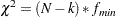
where
is the function value at the minimum, is the total sample size, and is the number of independent groups. The associated degrees of freedom is denoted by . For the ML estimation, this gives the likelihood ratio test statistic of the specified structural model in the null hypothesis against an unconstrained saturated model in the alternative hypothesis. The
test is valid only if the observations are independent and identically distributed, the analysis is based on the unstandardized sample covariance matrix  , and the sample size is sufficiently large (Browne; 1982; Bollen; 1989b; Jöreskog and Sörbom; 1985). For ML and GLS estimates, the variables must also have an approximately multivariate normal distribution.
 In the output fit summary table of PROC CALIS, the notation "Prob > Chi-Square" means "the probability of obtaining a greater
value than the observed value under the null hypothesis." This probability is also known as the -value of the chi-square test statistic. adjusted
value (Browne; 1982)
If the variables are-variate elliptic rather than normal and have significant amounts of multivariate kurtosis (leptokurtic or platykurtic), the value can be adjusted to: 
where
 is the multivariate relative kurtosis coefficient.
 Z-test (Wilson and Hilferty; 1931)
The Z-test of Wilson and Hilferty assumes a-variate normal distribution: 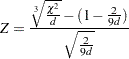
where
 is the degrees of freedom of the model. Refer to McArdle (1988) and Bishop, Fienberg, and Holland (1975, p. 527) for an application of the Z-test.
 critical N index (Hoelter; 1983)
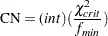
where
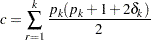
 is the critical chi-square value for the given degrees of freedom and probability
  , and int() takes the integer part of the expression. Refer to Bollen (1989b, p. 277). Hoelter (1983) suggests that CN should be at least 200; however, Bollen (1989b) notes that the CN value might lead to an overly pessimistic assessment of fit for small samples.
 root mean square residual (RMR)
For a single-group analysis, the RMR is the root of the mean of the squared residuals: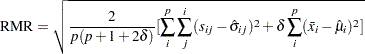
For multiple-group analysis, PROC CALIS computes the root mean square residual
 for each group first. To obtain an overall RMR measure for the analysis, individual ’s are weighted by the group weights
  . That is,
standardized root mean square residual (SRMR)
For a single-group analysis, the SRMR is the root of the mean of the squared standardized residuals: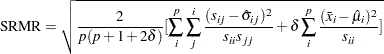
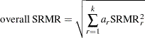
Similar to the calculation of the overall RMR, an overall measure of SRMR in a multiple-group analysis is a weighted average of the individual SRMR’s. That is, with
goodness-of-fit index (GFI)
For a single-group analysis, the goodness-of-fit index for the ULS, GLS, and ML estimation methods is:
with
 for ULS,
  for GLS, and
  . For WLS and DWLS estimation,
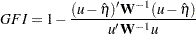
where
 is the vector of observed moments and
  is the vector of fitted moments. When the mean structures are modeled, vectors and contains all the nonredundant elements
  in the covariance matrix and all the means. That is,
and the symmetric weight matrix
is of dimension  . When the mean structures are not modeled, vectors and contains all the nonredundant elements in the covariance matrix only. That is,
and the symmetric weight matrix
is of dimension  . In addition, for the DWLS estimation, is a diagonal matrix.
 For a constant weight matrix
, the goodness-of-fit index is 1 minus the ratio of the minimum function value and the function value before any model has been fitted. The GFI should be between 0 and 1. The data probably do not fit the model if the GFI is negative or much larger than 1. For a multiple-group analysis, individual
 ’s are computed for groups. The overall measure is a weighted average of individual ’s, using weight . That is,
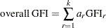
Parsimony Indices
These indices are constructed so that the model complexity is taken into account when assessing model fit. In general, models with more parameters (fewer degrees of freedom) are penalized.
adjusted goodness-of-fit index (AGFI)
The AGFI is the GFI adjusted for the degrees of freedom of the model, 
where
computes the total number of elements in the covariance matrices and mean vectors for modeling. For single-group analyses, the AGFI corresponds to the GFI in replacing the total sum of squares by the mean sum of squares.
Caution:
Large
and small can result in a negative AGFI. For example, GFI , p
, p , and d
 result in an AGFI of
  .
. AGFI is not defined for a saturated model, due to division by
 .
. AGFI is not sensitive to losses in
.
The AGFI should be between 0 and 1. The data probably do not fit the model if the AGFI is negative or much larger than 1. For more information, refer to Mulaik et al. (1989).
parsimonious goodness-of-fit index (PGFI)
The PGFI (Mulaik et al.; 1989) is a modification of the GFI that takes the parsimony of the model into account: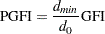
where
is the model degrees of freedom and  is the degrees of freedom for the independence model. See the section Incremental Indices for the definition of independence model. The PGFI uses the same parsimonious factor as the parsimonious normed Bentler-Bonett index (James, Mulaik, and Brett; 1982).
 RMSEA index (Steiger and Lind; 1980; Steiger; 1998)
The root mean square error approximation (RMSEA) coefficient is: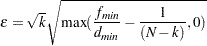
The lower and upper limits of the
 -confidence interval are computed using the cumulative distribution function of the noncentral chi-squared distribution
  . With
  ,
,  satisfying
 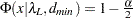 , and
, and  satisfying
  :
: 
Refer to Browne and Du Toit (1992) for more details. The size of the confidence interval can be set by the option ALPHARMS=
 ,
,  . The default is
  , which corresponds to the 90% confidence interval for the RMSEA.
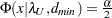
 probability for test of close fit (Browne and Cudeck; 1993)
The traditional exact test hypothesis  is replaced by the null hypothesis of close fit
  and the exceedance probability
  is computed as:
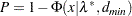
where
and 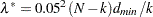 . The null hypothesis of close fit is rejected if is smaller than a pre-specified level (for example,
  ).
). ECVI: expected cross validation index (Browne and Cudeck; 1993)
The following formulas for ECVI are limited to the case of single-sample analysis without mean structures. For other cases, ECVI is not defined in PROC CALIS. For GLS and WLS, the estimator of the ECVI is linearly related to AIC, Akaike’s Information Criterion (Akaike; 1974, 1987):
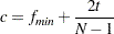
For ML estimation,
 is used:
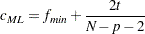
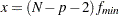
For GLS and WLS, the confidence interval
 for ECVI is computed using the cumulative distribution function
  of the noncentral chi-squared distribution,
with
 ,
,  , and
, and  .
. For ML, the confidence interval
 for ECVI is:
where
 ,
, 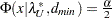 and
and 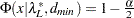 . Refer to Browne and Cudeck (1993). The size of the confidence interval can be set by the option ALPHAECV=, . The default is , which corresponds to the 90% confidence interval for the ECVI.
 Akaike’s information criterion (AIC) (Akaike; 1974, 1987)
This is a criterion for selecting the best model among a number of candidate models. The model that yields the smallest value of AIC is considered the best.
where
 is the
  times the likelihood function value for the FIML method or the value for other estimation methods.
 consistent Akaike’s information criterion (CAIC) (Bozdogan; 1987)
This is another criterion, similar to AIC, for selecting the best model among alternatives. The model that yields the smallest value of CAIC is considered the best. CAIC is preferred by some people to AIC or the test. 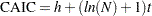
where
is the times the likelihood function value for the FIML method or the value for other estimation methods. Notice that includes the number of incomplete observations for the FIML method while it includes only the complete observations for other estimation methods. Schwarz’s Bayesian criterion (SBC) (Schwarz; 1978; Sclove; 1987)
This is another criterion, similar to AIC, for selecting the best model. The model that yields the smallest value of SBC is considered the best. SBC is preferred by some people to AIC or the test. 
where
is the times the likelihood function value for the FIML method or the value for other estimation methods. Notice that includes the number of incomplete observations for the FIML method while it includes only the complete observations for other estimation methods. McDonald’s measure of centrality (McDonald and Marsh; 1988)
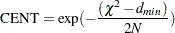
Incremental Indices
These indices are constructed so that the model fit is assessed through the comparison with a baseline model. The baseline model is usually the independence model where all covariances among manifest variables are assumed to be zeros. The only parameters in the independence model are the diagonals of covariance matrix. If modeled, the mean structures are saturated in the independence model. For multiple-group analysis, the overall independence model consists of component independence models for each group.
In the following, let  and denote the minimized discrepancy function value and the associated degrees of freedom, respectively, for the independence model; and and denote the minimized discrepancy function value and the associated degrees of freedom, respectively, for the model being fitted in the null hypothesis.
Bentler comparative fit index (Bentler; 1995)

Bentler-Bonett normed fit index (NFI) (Bentler and Bonett; 1980)

Mulaik et al. (1989) recommend the parsimonious weighted form called parsimonious normed fit index (PNFI) (James, Mulaik, and Brett; 1982).
Bentler-Bonett nonnormed coefficient (Bentler and Bonett; 1980)
Refer to Tucker and Lewis (1973).
normed index
 (Bollen; 1986)
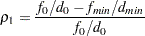
 is always less than or equal to
  ;
;  is unlikely in practice. Refer to the discussion in Bollen (1989a).
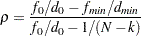
 nonnormed index
 (Bollen; 1989a)
is a modification of Bentler and Bonett’s
 that uses and "lessens the dependence" on . Refer to the discussion in (Bollen; 1989b).
  is identical to the IFI2 index of Mulaik et al. (1989).
 parsimonious normed fit index (James, Mulaik, and Brett; 1982)
The PNFI is a modification of Bentler-Bonett’s normed fit index that takes parsimony of the model into account,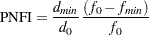
The PNFI uses the same parsimonious factor as the parsimonious GFI of Mulaik et al. (1989).
Fit Indices and Estimation Methods
Note that not all fit indices are reasonable or appropriate for all estimation methods set by the METHOD= option of the PROC CALIS statement. The availability of fit indices is summarized as follows:
Adjusted (elliptic) chi-square and its probability are available only for METHOD=ML or GLS and with the presence of raw data input.
For METHOD=ULS or DWLS, probability of the chi-square value, RMSEA and its confidence intervals, probability of close fit, ECVI and its confidence intervals, critical N index, Z-test, AIC, CAIC, SBC, and measure of centrality are not appropriate and therefore not displayed.
Individual Fit Indices for Multiple Groups
When you compare the fits of individual groups in a multiple-group analysis, you can examine the residuals of the groups to gauge which group is fitted better than the others. While examining residuals is good for knowing specific locations with inadequate fit, summary measures like fit indices for individual groups would be more convenient for overall comparisons among groups.
Although the overall fit function is a weighted sum of individual fit functions for groups, these individual functions are not statistically independent. Therefore, in general you cannot partition the degrees of freedom or value according to the groups. This eliminates the possibility of breaking down those fit indices that are functions of degrees of freedom or for group comparison purposes. Bearing this fact in mind, PROC CALIS computes only a limited number of descriptive fit indices for individual groups.
fit function
The overall fit function is:where
and are the group weight and the discrepancy function for group , respectively. The value of unweighted fit function for the -th group is denoted by: 
This
 value provides a measure of fit in the -th group without taking the sample size into account. The large the , the worse the fit for the group.
 percentage contribution to the chi-square
The percentage contribution of group to the chi-square is: 
where
is the value of with minimized at the value . This percentage value provides a descriptive measure of fit of the moments in group , weighted by its sample size. The group with the largest percentage contribution accounts for the most lack of fit in the overall model. root mean square residual (RMR)
For the-th group, the total number of moments being modeled is: 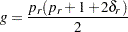
where
is the number of variables and is the indicator variable of the mean structures in the -th group. The root mean square residual for the -th group is: 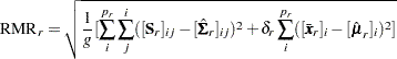
standardized root mean square residual (SRMR)
For the-th group, the standardized root mean square residual is: 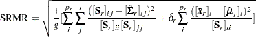
goodness-of-fit index (GFI)
For the ULS, GLS, and ML estimation, the goodness-of-fit index (GFI) for the-th group is: 
with
 for ULS,
  for GLS, and
  . For the WLS and DWLS estimation,
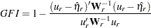
where
 is the vector of observed moments and
  is the vector of fitted moments for the -th group (
 ).
). When the mean structures are modeled, vectors
and  contain all the nonredundant elements
  in the covariance matrix and all the means, and is the weight matrix for covariances and means. When the mean structures are not modeled, , , and contain elements pertaining to the covariance elements only. Basically, formulas presented here are the same as the case for a single-group GFI. The only thing added here is the subscript to denote individual group measures.
 Bentler-Bonnett normed fit index (NFI)
For the-th group, the Bentler-Bonnett NFI is: 
where
 is the function value for fitting the independence model to the -th group. The larger the value of
  , the better is the fit for the group. Basically, the formula here is the same as the overall Bentler-Bonnet NFI. The only difference is that the subscript is added to denote individual group measures.
Squared Multiple Correlations and Determination Coefficients
In the section, squared multiple correlations for endogenous variables are defined. Squared multiple correlation is computed for all of these five estimation methods: ULS, GLS, ML, WLS, and DWLS. These coefficients are also computed as in the LISREL VI program of Jöreskog and Sörbom (1985). The DETAE, DETSE, and DETMV determination coefficients are intended to be multivariate generalizations of the squared multiple correlations for different subsets of variables. These coefficients are displayed only when you specify the PDETERM option.
 values corresponding to endogenous variables
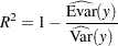
where
 denotes an endogenous variable,
  denotes its variance, and
  denotes its error (or unsystematic) variance. The variance and error variance are estimated under the model.
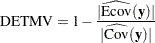
 total determination of all equations

where the
 vector denotes all manifest dependent variables, the
  vector denotes all latent dependent variables,
  denotes the covariance matrix of and , and
  denotes the error covariance matrix of and . The covariance matrices are estimated under the model.
 total determination of latent equations
where the
vector denotes all latent dependent variables,  denotes the covariance matrix of , and
  denotes the error covariance matrix of . The covariance matrices are estimated under the model.
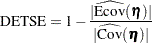
 total determination of the manifest equations
where the
vector denotes all manifest dependent variables,  denotes the covariance matrix of ,
  denotes the error covariance matrix of , and
  denotes the determinant of matrix
  . All the covariance matrices in the formula are estimated under the model.
You can also use the DETERM statement to request the computations of determination coefficients for any subsets of dependent variables.
Copyright © SAS Institute, Inc. All Rights Reserved.