In many applications, the manifest variables are not even approximately multivariate normal. If this happens to be the case with your data set, the default generalized least squares and maximum likelihood estimation methods are not appropriate, and you should compute the parameter estimates and their standard errors by an asymptotically distribution-free method, such as the WLS estimation method. If your manifest variables are multivariate normal, then they have a zero relative multivariate kurtosis, and all marginal distributions have zero kurtosis (Browne; 1982). If your DATA= data set contains raw data, PROC CALIS computes univariate skewness and kurtosis and a set of multivariate kurtosis values. By default, the values of univariate skewness and kurtosis are corrected for bias (as in PROC UNIVARIATE), but using the BIASKUR option enables you to compute the uncorrected values also. The values are displayed when you specify the PROC CALIS statement option KURTOSIS.

In the following formulas, denotes the sample size and denotes the number of variables.

• corrected variance for variable
  

• uncorrected univariate skewness for variable
  

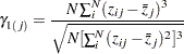
• corrected univariate skewness for variable
  

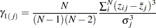
• uncorrected univariate kurtosis for variable
  

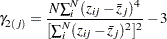
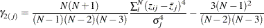
• corrected univariate kurtosis for variable
  

• Mardia’s multivariate kurtosis
  

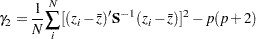
  where is the biased sample covariance matrix with as the divisor.

• relative multivariate kurtosis
  

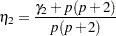
• normalized multivariate kurtosis
  

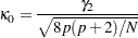
• Mardia based kappa
  

• mean scaled univariate kurtosis
  

• adjusted mean scaled univariate kurtosis
  

  with

If variable is normally distributed, the uncorrected univariate kurtosis is equal to 0. If has an -variate normal distribution, Mardia’s multivariate kurtosis is equal to 0. A variable is called leptokurtic if it has a positive value of and is called platykurtic if it has a negative value of . The values of , , and should not be smaller than the following lower bound (Bentler; 1985):

PROC CALIS displays a message if , , or falls below the lower bound.

If weighted least squares estimates (METHOD=WLS or METHOD=ADF) are specified and the weight matrix is computed from an input raw data set, the CALIS procedure computes two more measures of multivariate kurtosis.

• multivariate mean kappa
  

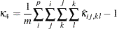
  where

  and is the number of elements in the vector (Bentler; 1985).

• multivariate least squares kappa
  

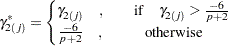
  where is the vector of the elements in the denominator of (Bentler; 1985) and is the vector of the , which is defined as:

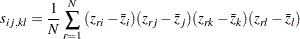
The occurrence of significant nonzero values of Mardia’s multivariate kurtosis and significant amounts of some of the univariate kurtosis values indicate that your variables are not multivariate normal distributed. Violating the multivariate normality assumption in (default) generalized least squares and maximum likelihood estimation usually leads to the wrong approximate standard errors and incorrect fit statistics based on the value. In general, the parameter estimates are more stable against violation of the normal distribution assumption. For more details, refer to Browne (1974, 1982, 1984).