The HPSPLIT Procedure

Example 16.4 Creating a Binary Classification Tree with Validation Data
A common use of classification trees is to predict the likelihood that a mortgage applicant will default on a loan. The data
set Hmeq, which is in the Sampsio library that SAS provides, contains observations for 5,960 mortgage applicants. A variable named Bad indicates whether the applicant paid or defaulted on the loan that was given.
This example uses Hmeq to build a tree model that is used to score the data and can be used to score data about new applicants. Table 16.6 describes the variables in Hmeq.
Table 16.6: Variables in the Home Equity (Hmeq) Data Set
|
Variable |
Role |
Level |
Description |
|---|---|---|---|
|
|
Response |
Binary |
1 = applicant defaulted on the loan or is seriously delinquent |
|
0 = applicant paid the loan |
|||
|
|
Predictor |
Interval |
Age of oldest credit line in months |
|
|
Predictor |
Interval |
Number of credit lines |
|
|
Predictor |
Interval |
Debt-to-income ratio |
|
|
Predictor |
Interval |
Number of delinquent credit lines |
|
|
Predictor |
Interval |
Number of major derogatory reports |
|
|
Predictor |
Nominal |
Occupational category |
|
|
Predictor |
Interval |
Requested loan amount |
|
|
Predictor |
Interval |
Amount due on existing mortgage |
|
|
Predictor |
Interval |
Number of recent credit inquiries |
|
|
Predictor |
Binary |
|
|
|
|||
|
|
Predictor |
Interval |
Value of current property |
|
|
Predictor |
Interval |
Years at present job |
The response variable for the tree model is Bad, a class variable that has two values (0 indicates payment of loan, and 1 indicates default). The other variables are predictor
variables for the model. The following statements display the first 10 observations of the data set:
/* Convert variable names to mixed case */
data hmeq;
   length Bad Loan MortDue Value 8 Reason Job $7
          YoJ Derog Delinq CLAge nInq CLNo DebtInc 8;
   set sampsio.hmeq;
run;

proc print data=hmeq(obs=10); run;
Output 16.4.1 shows the partial listing of Hmeq.
Output 16.4.1: Partial Listing of the Hmeq Data
| Obs | Bad | Loan | MortDue | Value | Reason | Job | YoJ | Derog | Delinq | CLAge | nInq | CLNo | DebtInc |
|---|---|---|---|---|---|---|---|---|---|---|---|---|---|
| 1 | 1 | 1100 | 25860 | 39025 | HomeImp | Other | 10.5 | 0 | 0 | 94.367 | 1 | 9 | . |
| 2 | 1 | 1300 | 70053 | 68400 | HomeImp | Other | 7.0 | 0 | 2 | 121.833 | 0 | 14 | . |
| 3 | 1 | 1500 | 13500 | 16700 | HomeImp | Other | 4.0 | 0 | 0 | 149.467 | 1 | 10 | . |
| 4 | 1 | 1500 | . | . | . | . | . | . | . | . | . | ||
| 5 | 0 | 1700 | 97800 | 112000 | HomeImp | Office | 3.0 | 0 | 0 | 93.333 | 0 | 14 | . |
| 6 | 1 | 1700 | 30548 | 40320 | HomeImp | Other | 9.0 | 0 | 0 | 101.466 | 1 | 8 | 37.1136 |
| 7 | 1 | 1800 | 48649 | 57037 | HomeImp | Other | 5.0 | 3 | 2 | 77.100 | 1 | 17 | . |
| 8 | 1 | 1800 | 28502 | 43034 | HomeImp | Other | 11.0 | 0 | 0 | 88.766 | 0 | 8 | 36.8849 |
| 9 | 1 | 2000 | 32700 | 46740 | HomeImp | Other | 3.0 | 0 | 2 | 216.933 | 1 | 12 | . |
| 10 | 1 | 2000 | . | 62250 | HomeImp | Sales | 16.0 | 0 | 0 | 115.800 | 0 | 13 | . |
The following statements use the HPSPLIT procedure to create a classification tree:
ods graphics on;

proc hpsplit data=hmeq maxdepth=5;
   class Bad Delinq Derog Job nInq Reason;
   model Bad(event='1') = Delinq Derog Job nInq Reason CLAge CLNo
               DebtInc Loan MortDue Value YoJ;
   prune costcomplexity;
   partition fraction(validate=0.3 seed=123);
   code file='hpsplexc.sas';
   rules file='rules.txt';
run;
The MAXDEPTH= option specifies the maximum depth of the tree to be grown.
Specifying Bad to the left of the equal sign in the MODEL
statement indicates that it is the response variable. Because Bad is a binary response, the EVENT= option specifies that the calculations for sensitivity, specificity, AUC, and ROC be based
on the level Bad=1.
By default, the entropy metric is used to grow the tree. The PRUNE statement requests cost-complexity pruning.
The PARTITION
statement specifies that the observations in Hmeq be logically partitioned into disjoint subsets for model training and validation. Observations are randomly selected for
the validation subset with the probability 0.3; the remaining observations are selected for the training subset.
The FILE= option in the CODE
statement requests that SAS DATA step score code be saved to a file named hpsplexc.sas, and the FILE= option in the RULES
statement requests that the node rules be saved to a file named rules.txt.
The tree diagram in Output 16.4.2 provides an overview of the full tree.
Output 16.4.2: Overview Diagram of Final Tree
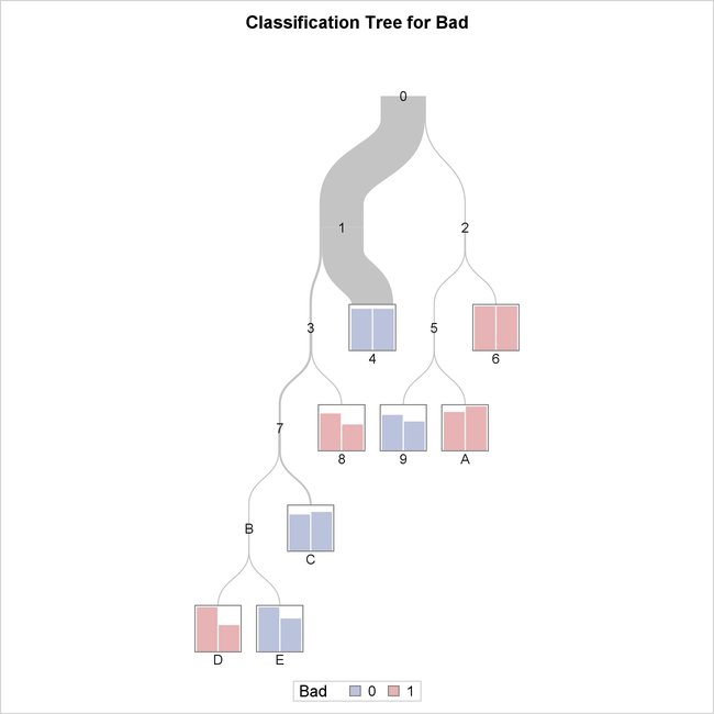
You can see from this diagram that the observations in terminal nodes 4, 9, C, and E are assigned a prediction of Bad=0 and those in terminal nodes 6, 8, A, and D are assigned a prediction of Bad=1. You can easily see that node 4 contains the most observations, as indicated by thickness of the link from its parent node.
The tree diagram in Output 16.4.3 is a detailed view of the top portion of the tree. You can use the PLOTS= option in the PROC HPSPLIT statement to control which nodes are displayed.
Output 16.4.3: Detailed Tree Diagram
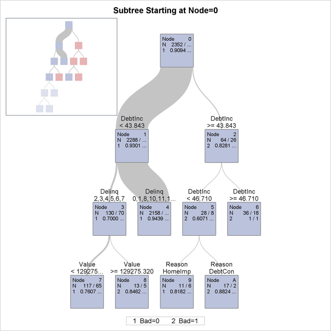
By default, this view provides detailed splitting information about the first three levels of the tree, including the splitting
variable and splitting values. The splitting rule above each node determines which observations from the parent node are included
in the node. The first row of the table inside the node provides the node identifier. The second row of the table provides
the number of training and validation observations, separated by a slash. The third row shows the predicted response for observations
in that node if classification was occurring at that point, along with the proportion of training and validation observations
with that observed response. Note that the legend shows what actual value of the response variable is represented by the value
shown in the node. For example, in node 6, all 36 observations in the training data and all 18 observations in the validation
data have an observed response value of Bad=1, as indicated by the value 2 shown on the third line.
Because the response is categorical, the confusion matrices for the training data and for the validation data are displayed in the table shown in Output 16.4.4.
Output 16.4.4: Training and Validation Confusion Matrices
For the training data, there are 73 observations where the model correctly predicted Bad=1 and 2,135 observations where the model correctly predicted Bad=0. The values in the off-diagonal entries of the matrices show how many times the model misclassified observations.
When you are modeling a binary response variable, a plot of the ROC curve is displayed as shown in Output 16.4.5.
Output 16.4.5: ROC Plot
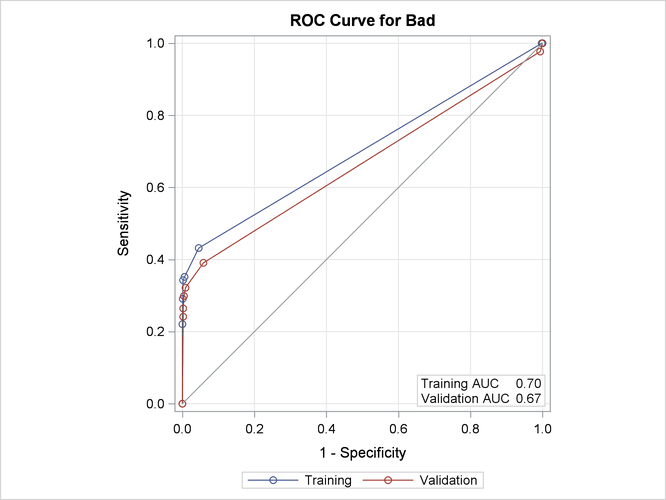
This plot summarizes the performance of the tree model in terms of sensitivity and specificity.
Output 16.4.6 displays the "Tree Performance" table, which provides several impurity measures and fit statistics for the final tree.
Output 16.4.6: Tree Performance
The last three columns of this table contain statistics related to the ROC curve plotted in Output 16.4.5. This model does not classify the observations with Bad=1 (the event of interest) very well, as you can see in the confusion matrix and from the low sensitivity reported in this
table. This is often the case with a relatively rare event. The AUC measures the area under the ROC curve. A model that fits
the data perfectly would have an AUC of 1. These three columns are included only for a binary response variable.
Output 16.4.7 displays the pruning plot.
Output 16.4.7: Pruning Plot
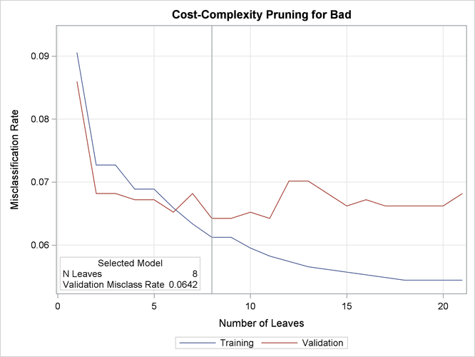
This plot displays misclassification rates for the training and validation data as the tree is pruned. The tree with eight leaves is selected as the final tree because it has the lowest misclassification rate for the validation data.
Creating Score Code and Scoring New Data
In addition to seeing information about the tree model, you might be interested in applying a model to predict the response
variable in other data sets where the response is unknown. The following statements show how you can use the score code file
hpsplexc.sas, created by the FILE= option in the CODE statement, to score the data in Hmeq and save the results in a SAS data set named Scored.
data scored;
   set hmeq;
   %include 'hpsplexc.sas';
run;
Output 16.4.8 shows a partial listing of Scored.
Output 16.4.8: Partial Listing of the Scored Hmeq Data
| Obs | Bad | Loan | MortDue | Value | Reason | Job | YoJ | Derog | Delinq | CLAge | nInq | CLNo | DebtInc | _Node_ | _Leaf_ | _WARN_ | P_Bad0 | P_Bad1 | V_Bad0 | V_Bad1 |
|---|---|---|---|---|---|---|---|---|---|---|---|---|---|---|---|---|---|---|---|---|
| 1 | 1 | 1100 | 25860 | 39025 | HomeImp | Other | 10.5 | 0 | 0 | 94.367 | 1 | 9 | . | 4 | 0 | 0.94393 | 0.05607 | 0.94432 | 0.05568 | |
| 2 | 1 | 1300 | 70053 | 68400 | HomeImp | Other | 7.0 | 0 | 2 | 121.833 | 0 | 14 | . | 12 | 5 | 0.83168 | 0.16832 | 0.88462 | 0.11538 | |
| 3 | 1 | 1500 | 13500 | 16700 | HomeImp | Other | 4.0 | 0 | 0 | 149.467 | 1 | 10 | . | 4 | 0 | 0.94393 | 0.05607 | 0.94432 | 0.05568 | |
| 4 | 1 | 1500 | . | . | . | . | . | . | . | . | . | 4 | 0 | 0.94393 | 0.05607 | 0.94432 | 0.05568 | |||
| 5 | 0 | 1700 | 97800 | 112000 | HomeImp | Office | 3.0 | 0 | 0 | 93.333 | 0 | 14 | . | 4 | 0 | 0.94393 | 0.05607 | 0.94432 | 0.05568 | |
| 6 | 1 | 1700 | 30548 | 40320 | HomeImp | Other | 9.0 | 0 | 0 | 101.466 | 1 | 8 | 37.1136 | 4 | 0 | 0.94393 | 0.05607 | 0.94432 | 0.05568 | |
| 7 | 1 | 1800 | 48649 | 57037 | HomeImp | Other | 5.0 | 3 | 2 | 77.100 | 1 | 17 | . | 12 | 5 | 0.83168 | 0.16832 | 0.88462 | 0.11538 | |
| 8 | 1 | 1800 | 28502 | 43034 | HomeImp | Other | 11.0 | 0 | 0 | 88.766 | 0 | 8 | 36.8849 | 4 | 0 | 0.94393 | 0.05607 | 0.94432 | 0.05568 | |
| 9 | 1 | 2000 | 32700 | 46740 | HomeImp | Other | 3.0 | 0 | 2 | 216.933 | 1 | 12 | . | 12 | 5 | 0.83168 | 0.16832 | 0.88462 | 0.11538 | |
| 10 | 1 | 2000 | . | 62250 | HomeImp | Sales | 16.0 | 0 | 0 | 115.800 | 0 | 13 | . | 4 | 0 | 0.94393 | 0.05607 | 0.94432 | 0.05568 |
The data set contains the 13 original variables and the 7 new variables that are created by the score code. The variable P_Bad1 is the proportion of training observations on this leaf for which Bad=1, and this variable can be interpreted as the probability of default. The variable V_Bad1 is the proportion of validation observations on this leaf for which Bad=1. Similar variables are created for the other response value, Bad=0. Also included in the scored data set are the node and leaf assignments, which are shown in the variables _Node_ and _Leaf_, respectively. Note that these same variables are included in the OUT= data set when you specify that option in the OUTPUT statement
. For more information about these variables, see the section Scoring.
You can use the preceding statements to score new data by including the new data set in place of Hmeq in the SET statement. The new data set must contain the same variables as the data that are used to build the tree model,
but not the unknown response variable that you are now trying to predict.
Creating a Node Rules Description of a Tree
When you specify the FILE= option in the RULES
statement, a file that contains the node rules is created. In this example, PROC HPSPLIT saves the node rules of the tree
model to a file named rules.txt; a partial listing of this file is shown in Output 16.4.9.
Output 16.4.9: Rules File
*------------------------------------------------------------*
NODE = 4
*------------------------------------------------------------*
MISSING(Delinq) OR (Delinq IS ONE OF 0, 1, 8, 10, 11, 12, 13, 15)
AND MISSING(DebtInc) OR (DebtInc < 43.843383)
    PREDICTED VALUE IS 0
    PREDICTED 0 = 0.9439( 2037/2158)
    PREDICTED 1 = 0.05607( 121/2158)
*------------------------------------------------------------*
NODE = 13
*------------------------------------------------------------*
MISSING(CLNo) OR (CLNo < 30.08)
AND (Delinq IS ONE OF 4, 5, 6, 7)
AND MISSING(Value) OR (Value < 129275.32)
AND (Delinq IS ONE OF 2, 3, 4, 5, 6, 7)
AND MISSING(DebtInc) OR (DebtInc < 43.843383)
    PREDICTED VALUE IS 1
    PREDICTED 0 = 0( 0/11)
    PREDICTED 1 = 1( 11/11)
*------------------------------------------------------------*
NODE = 14
*------------------------------------------------------------*
(CLNo >= 30.08)
AND (Delinq IS ONE OF 4, 5, 6, 7)
AND MISSING(Value) OR (Value < 129275.32)
AND (Delinq IS ONE OF 2, 3, 4, 5, 6, 7)
AND MISSING(DebtInc) OR (DebtInc < 43.843383)
    PREDICTED VALUE IS 0
    PREDICTED 0 = 1( 5/5)
    PREDICTED 1 = 0( 0/5)
*------------------------------------------------------------*
NODE = 9
*------------------------------------------------------------*
(Reason IS HomeImp)
AND (DebtInc < 46.7104)
AND (DebtInc >= 43.843383)
    PREDICTED VALUE IS 0
    PREDICTED 0 = 0.8182( 9/11)
    PREDICTED 1 = 0.1818( 2/11)
|
In this listing, the predicted value and the fraction of observations for each level of the response variable are displayed for each terminal node. The nodes are not numbered consecutively because only terminal nodes (leaves) are included. The splits that lead to each leaf are shown above the predicted value and fractions.