The HPLMIXED Procedure

Estimating Fixed and Random Effects in the Mixed Model
ML and REML methods provide estimates of  and
and  , which are denoted
  and
and  , respectively. To obtain estimates of
  and predicted values of
  , the standard method is to solve the mixed model equations (Henderson 1984):
![\[ \left[\begin{array}{lr} \bX ’\widehat{\bR }^{-1}\bX & \bX ’\widehat{\bR }^{-1}\bZ \\*\bZ ’\widehat{\bR }^{-1}\bX & \bZ ’\widehat{\bR }^{-1}\bZ + \widehat{\bG }^{-1} \end{array}\right] \left[\begin{array}{c} \widehat{\bbeta } \\ \widehat{\bgamma } \end{array} \right] = \left[\begin{array}{r} \bX ’\widehat{\bR }^{-1}\mb{y} \\ \bZ ’\widehat{\bR }^{-1}\mb{y} \end{array} \right] \]](images/stathpug_hplmixed0191.png)
The solutions can also be written as
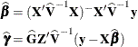
and have connections with empirical Bayes estimators (Laird and Ware 1982; Carlin and Louis 1996). Note that the are random variables and not parameters (unknown constants) in the model. Technically, determining values for from the data is thus a prediction task, whereas determining values for is an estimation task.
The mixed model equations are extended normal equations. The preceding expression assumes that is nonsingular. For the extreme case where the eigenvalues of are very large,  contributes very little to the equations and
  is close to what it would be if actually contained fixed-effects parameters. On the other hand, when the eigenvalues of are very small, dominates the equations and is close to 0. For intermediate cases, can be viewed as shrinking the fixed-effects estimates of toward 0 (Robinson 1991).
If is singular, then the mixed model equations are modified (Henderson 1984) as follows:
![\[ \left[\begin{array}{lr} \bX ’\widehat{\bR } ^{-1}\bX & \bX ’\widehat{\bR } ^{-1} \bZ \widehat{\bG } \\ \widehat{\bG }’\bZ ’\widehat{\bR } ^{-1}\bX & \widehat{\bG }’\bZ ’\widehat{\bR } ^{-1}\bZ \widehat{\bG } + \bG \end{array}\right] \left[\begin{array}{c} \widehat{\bbeta } \\ \widehat{\btau } \end{array} \right] = \left[\begin{array}{r} \bX ’\widehat{\bR } ^{-1}\mb{y} \\ \widehat{\bG }’\bZ ’\widehat{\bR } ^{-1}\mb{y} \end{array} \right] \]](images/stathpug_hplmixed0194.png)
Denote the generalized inverses of the nonsingular and singular forms of the mixed model equations by  and
and  , respectively. In the nonsingular case, the solution estimates the random effects directly. But in the singular case, the estimates of random effects are achieved through a back-transformation
 where
where  is the solution to the modified mixed model equations. Similarly, while in the nonsingular case itself is the estimated covariance matrix for
  , in the singular case the covariance estimate for
  is given by
  where
where
![\[ \bP = \left[\begin{array}{cc} \bI & \\ & \widehat{\bG } \end{array}\right] \]](images/stathpug_hplmixed0202.png)
An example of when the singular form of the equations is necessary is when a variance component estimate falls on the boundary constraint of 0.