The HPLMIXED Procedure

RANDOM Statement

RANDOM random-effects </ options>;

The RANDOM statement defines the random effects that constitute the $\bgamma$ vector in the mixed model. You can use this statement to specify traditional variance component models and to specify random coefficients. The random effects can be classification or continuous, and multiple RANDOM statements are possible.

Using notation from the section Linear Mixed Models Theory, the purpose of the RANDOM statement is to define the $\mb{Z}$ matrix of the mixed model, the random effects in the $\bgamma$ vector, and the structure of $\mb{G}$ . The $\mb{Z}$ matrix is constructed exactly as the $\mb{X}$ matrix for the fixed effects is constructed, and the $\mb{G}$ matrix is constructed to correspond with the effects that constitute $\mb{Z}$ . The structure of $\mb{G}$ is defined by using the TYPE= option.

You can specify INTERCEPT (or INT) as a random effect to indicate the intercept. PROC HPLMIXED does not include the intercept in the RANDOM statement by default as it does in the MODEL statement.

Table 9.5 summarizes important options in the RANDOM statement. All options are subsequently discussed in alphabetical order.

Table 9.5: Summary of Important RANDOM Statement Options

Option	Description
Construction of Covariance Structure
SUBJECT=	Identifies the subjects in the model
TYPE=	Specifies the covariance structure
Statistical Output
ALPHA= $\alpha$	Determines the confidence level ( $1-\alpha$ )
CL	Requests confidence limits for predictors of random effects
SOLUTION	Displays solutions $\widehat{\bgamma }$ of the random effects

You can specify the following options in the RANDOM statement after a slash (/).

ALPHA=number

sets the confidence level to be $1-$ number for each confidence interval of the random-effects estimates. The value of number must be between 0 and 1; the default is 0.05.

CL

requests that t-type confidence limits be constructed for each of the random-effect estimates. The confidence level is 0.95 by default; this can be changed with the ALPHA= option.

SOLUTION S

requests that the solution for the random-effects parameters be produced. Using notation from the section Linear Mixed Models Theory, these estimates are the empirical best linear unbiased predictors (EBLUPs), 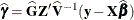$\widehat{\bgamma } = \widehat{\mb{G}}\mb{Z}’\widehat{\mb{V}}^{-1}(\mb{y} - \mb{X}\widehat{\bbeta })$ . They can be useful for comparing the random effects from different experimental units and can also be treated as residuals in performing diagnostics for your mixed model.

The numbers displayed in the SE Pred column of the "Solution for Random Effects" table are not the standard errors of the $\widehat{\bgamma }$ displayed in the Estimate column; rather, they are the standard errors of predictions $\widehat{\bgamma }_ i - \bgamma _ i$ , where $\widehat{\bgamma }_ i$ is the ith EBLUP and $\bgamma _ i$ is the ith random-effect parameter.

SUBJECT=effect SUB=effect

identifies the subjects in your mixed model. Complete independence is assumed across subjects; thus, for the RANDOM statement, the SUBJECT= option produces a block-diagonal structure in $\mb{G}$ with identical blocks. In fact, specifying a subject effect is equivalent to nesting all other effects in the RANDOM statement within the subject effect.

When you specify the SUBJECT= option and a classification random effect, computations are usually much quicker if the levels of the random effect are duplicated within each level of the SUBJECT= effect.

TYPE=covariance-structure

specifies the covariance structure of $\mb{G}$ . Valid values for covariance-structure and their descriptions are listed in Table 9.6. Although a variety of structures are available, most applications call for either TYPE=VC or TYPE=UN . The TYPE=VC (variance components) option is the default structure, and it models a different variance component for each random effect.

The TYPE=UN (unstructured) option is useful for correlated random coefficient models. For example, the following statement specifies a random intercept-slope model that has different variances for the intercept and slope and a covariance between them:

random intercept age / type=un subject=person;

You can also use TYPE=FA0(2) here to request a $\mb{G}$ estimate that is constrained to be nonnegative definite.

If you are constructing your own columns of $\mb{Z}$ with continuous variables, you can use the TYPE=TOEP (1) structure to group them together to have a common variance component. If you want to have different covariance structures in different parts of $\mb{G}$ , you must use multiple RANDOM statements with different TYPE= options.

Table 9.6: Covariance Structures

Structure	Description	Parms	$(i,j)$ element
ANTE(1)	Antedependence	$2t-1$	$\sigma _{i}\sigma _{j}\prod _{k=i}^{j-1}\rho _ k$
AR(1)	Autoregressive(1)	2	$\sigma ^2\rho ^{\|i-j\|}$
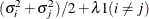
ARH(1)	Heterogeneous AR(1)	$t+1$	$\sigma _{i}\sigma _{j}\rho ^{\|i-j\|}$
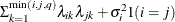
ARMA(1,1)	Autoregressive moving average(1,1)	3	$\sigma ^2[\gamma \rho ^{\|i-j\|-1} 1(i\neq j) + 1(i=j)]$
CS	Compound symmetry	2	$\sigma _1 + \sigma ^2 1(i=j)$
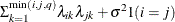
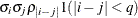
CSH	Heterogeneous compound symmetry	$t+1$	$\sigma _{i}\sigma _{j}[\rho 1(i \neq j)+ 1(i=j)]$
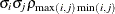
FA(q)	Factor analytic	$\frac{q}{2}(2t -q + 1) + t$	$\Sigma _{k=1}^{\min (i,j,q)} \lambda _{ik}\lambda _{jk}+\sigma ^2_ i 1(i=j)$
FA0(q)	No diagonal FA	$\frac{q}{2}(2t -q + 1)$	$\Sigma _{k=1}^{\min (i,j,q)} \lambda _{ik}\lambda _{jk}$
FA1(q)	Equal diagonal FA	$\frac{q}{2}(2t -q + 1) + 1$	$\Sigma _{k=1}^{\min (i,j,q)} \lambda _{ik}\lambda _{jk}+\sigma ^2 1(i=j)$
HF	Huynh-Feldt	$t+1$	$(\sigma _{i}^{2}+\sigma _{j}^{2})/2+\lambda 1(i\neq j)$
SIMPLE	An alias for VC	q	$\sigma ^2_ k 1(i=j)$ for the kth effect
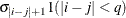
TOEP	Toeplitz	t	$\sigma _{\|i-j\|+1}$
TOEP(q)	Banded Toeplitz	q	$\sigma _{\|i-j\|+1} 1(\|i-j\|<q)$
TOEPH	Heterogeneous TOEP	$2t-1$	$\sigma _{i}\sigma _{j}\rho _{\|i-j\|}$
TOEPH(q)	Banded heterogeneous TOEP	$t+q-1$	$\sigma _{i}\sigma _{j}\rho _{\|i-j\|} 1(\|i-j\|<q)$
UN	Unstructured	$t(t+1)/2$	$\sigma _{ij}$
UN(q)	Banded	$\frac{q}{2}(2t-q+1)$	$\sigma _{ij} 1(\|i-j\|<q)$
UNR	Unstructured correlation	$t(t+1)/2$	$\sigma _{i}\sigma _{j}\rho _{\max (i,j)\min (i,j)}$
UNR(q)	Banded correlations	$\frac{q}{2}(2t-q+1)$	$\sigma _{i}\sigma _{j}\rho _{\max (i,j)\min (i,j)}$
VC	Variance components	q	$\sigma ^2_ k 1(i=j)$ for the kth effect

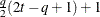
In Table 9.6, the Parms column represents the number of covariance parameters in the structure, t is the overall dimension of the covariance matrix, and $1(A)$ equals 1 when A is true and 0 otherwise. For example, 1 $(i=j)$ equals 1 when $i=j$ and 0 otherwise, and 1 $(|i-j|<q)$ equals 1 when $|i-j|<q$ and 0 otherwise. For the TYPE=TOEPH structures, $\rho _0 = 1$ ; for the TYPE=UNR structures, $\rho _{ii} = 1$ for all i.

Table 9.7 lists some examples of the structures in Table 9.6.

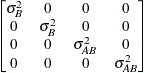
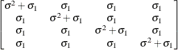
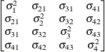
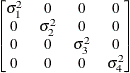
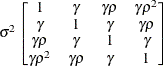
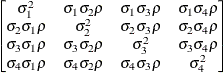
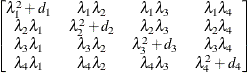
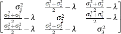
Table 9.7: Covariance Structure Examples

Description	Structure	Example
Variance components	VC (default)	$\begin{bmatrix} \sigma _{B}^{2} & 0 & 0 & 0 \\ 0 & \sigma _{B}^{2} & 0 & 0 \\ 0 & 0 & \sigma _{AB}^{2} & 0 \\ 0 & 0 & 0 & \sigma _{AB}^{2} \end{bmatrix}$
Compound symmetry	CS	$\begin{bmatrix} \sigma ^2 + \sigma _1 & \sigma _1 & \sigma _1 & \sigma _1 \\ \sigma _1 & \sigma ^2 + \sigma _1 & \sigma _1 & \sigma _1 \\ \sigma _1 & \sigma _1 & \sigma ^2 + \sigma _1 & \sigma _1 \\ \sigma _1 & \sigma _1 & \sigma _1 & \sigma ^2 + \sigma _1 \end{bmatrix}$
Unstructured	UN	$\begin{bmatrix} \sigma ^{2}_{1} & \sigma _{21} & \sigma _{31} & \sigma _{41} \\ \sigma _{21} & \sigma ^{2}_{2} & \sigma _{32} & \sigma _{42} \\ \sigma _{31} & \sigma _{32} & \sigma ^{2}_{3} & \sigma _{43} \\ \sigma _{41} & \sigma _{42} & \sigma _{43} & \sigma ^{2}_{4} \end{bmatrix}$
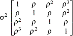
Banded main diagonal	UN(1)	$\begin{bmatrix} \sigma ^2_1 & 0 & 0 & 0 \\ 0 & \sigma ^2_2 & 0 & 0 \\ 0 & 0 & \sigma ^2_3 & 0 \\ 0 & 0 & 0 & \sigma ^2_4 \end{bmatrix}$
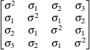
First-order autoregressive	AR(1)	$\sigma ^2\begin{bmatrix} 1 & \rho & \rho ^2 & \rho ^3 \\ \rho & 1 & \rho & \rho ^2 \\ \rho ^2 & \rho & 1 & \rho \\ \rho ^3 & \rho ^2 & \rho & 1 \end{bmatrix}$
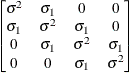
Toeplitz	TOEP	$\begin{bmatrix} \sigma ^2 & \sigma _1 & \sigma _2 & \sigma _3 \\ \sigma _1 & \sigma ^2 & \sigma _1 & \sigma _2 \\ \sigma _2 & \sigma _1 & \sigma ^2 & \sigma _1 \\ \sigma _3 & \sigma _2 & \sigma _1 & \sigma ^2 \end{bmatrix}$
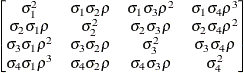
Toeplitz with two bands	TOEP(2)	$\begin{bmatrix} \sigma ^2 & \sigma _1 & 0 & 0 \\ \sigma _1 & \sigma ^2 & \sigma _1 & 0 \\ 0 & \sigma _1 & \sigma ^2 & \sigma _1 \\ 0 & 0 & \sigma _1 & \sigma ^2 \end{bmatrix}$
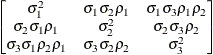
Heterogeneous autoregressive(1)	ARH(1)	$\begin{bmatrix} \sigma _{1}^{2} & \sigma _{1}\sigma _{2}\rho & \sigma _{1}\sigma _{3}\rho ^{2} & \sigma _{1}\sigma _{4}\rho ^{3} \\ \sigma _{2}\sigma _{1}\rho & \sigma _{2}^{2} & \sigma _{2}\sigma _{3}\rho & \sigma _{2}\sigma _{4}\rho ^{2} \\ \sigma _{3}\sigma _{1}\rho ^{2} & \sigma _{3}\sigma _{2}\rho & \sigma _{3}^{2} & \sigma _{3}\sigma _{4}\rho \\ \sigma _{4}\sigma _{1}\rho ^{3} & \sigma _{4}\sigma _{2}\rho & \sigma _{4}\sigma _{3}\rho & \sigma _{4}^{2} \end{bmatrix}$
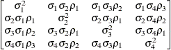
First-order autoregressive moving average	ARMA(1,1)	$\sigma ^2\begin{bmatrix} 1 & \gamma & \gamma \rho & \gamma \rho ^{2} \\ \gamma & 1 & \gamma & \gamma \rho \\ \gamma \rho & \gamma & 1 & \gamma \\ \gamma \rho ^{2} & \gamma \rho & \gamma & 1 \end{bmatrix}$
Heterogeneous compound symmetry	CSH	$\begin{bmatrix} \sigma _{1}^{2} & \sigma _{1}\sigma _{2}\rho & \sigma _{1}\sigma _{3}\rho & \sigma _{1}\sigma _{4}\rho \\ \sigma _{2}\sigma _{1}\rho & \sigma _{2}^{2} & \sigma _{2}\sigma _{3}\rho & \sigma _{2}\sigma _{4}\rho \\ \sigma _{3}\sigma _{1}\rho & \sigma _{3}\sigma _{2}\rho & \sigma _{3}^{2} & \sigma _{3}\sigma _{4}\rho \\ \sigma _{4}\sigma _{1}\rho & \sigma _{4}\sigma _{2}\rho & \sigma _{4}\sigma _{3}\rho & \sigma _{4}^{2} \end{bmatrix}$
First-order factor analytic	FA(1)	$\begin{bmatrix} \lambda _{1}^{2} + d_{1} & \lambda _{1}\lambda _{2} & \lambda _{1}\lambda _{3} & \lambda _{1}\lambda _{4} \\ \lambda _{2}\lambda _{1} & \lambda _{2}^{2} + d_{2} & \lambda _{2}\lambda _{3} & \lambda _{2}\lambda _{4} \\ \lambda _{3}\lambda _{1} & \lambda _{3}\lambda _{2} & \lambda _{3}^{2} + d_{3} & \lambda _{3}\lambda _{4} \\ \lambda _{4}\lambda _{1} & \lambda _{4}\lambda _{2} & \lambda _{4}\lambda _{3} & \lambda _{4}^{2} + d_{4} \end{bmatrix}$
Huynh-Feldt	HF	$\begin{bmatrix} \sigma _{1}^{2} & \frac{\sigma _{1}^{2}+\sigma _{2}^{2}}{2}-\lambda & \frac{\sigma _{1}^{2}+\sigma _{3}^{2}}{2}-\lambda \\ \frac{\sigma _{2}^{2}+\sigma _{1}^{2}}{2}-\lambda & \sigma _{2}^{2} & \frac{\sigma _{2}^{2}+\sigma _{3}^{2}}{2}-\lambda \\ \frac{\sigma _{3}^{2}+\sigma _{1}^{2}}{2}-\lambda & \frac{\sigma _{3}^{2}+\sigma _{2}^{2}}{2}-\lambda & \sigma _{3}^{2} \end{bmatrix}$
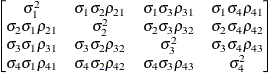
First-order antedependence	ANTE(1)	$\begin{bmatrix} \sigma ^2_1 & \sigma _1 \sigma _2 \rho _1 & \sigma _1 \sigma _3 \rho _1 \rho _2 \\ \sigma _2 \sigma _1 \rho _1 & \sigma ^2_2 & \sigma _2 \sigma _3 \rho _2 \\ \sigma _3 \sigma _1 \rho _2 \rho _1 & \sigma _3 \sigma _2 \rho _2 & \sigma ^2_3 \\ \end{bmatrix}$
Heterogeneous Toeplitz	TOEPH	$\begin{bmatrix} \sigma ^2_1 & \sigma _1 \sigma _2 \rho _1 & \sigma _1 \sigma _3 \rho _2 & \sigma _1 \sigma _4 \rho _3 \\ \sigma _2 \sigma _1 \rho _1 & \sigma ^2_2 & \sigma _2 \sigma _3 \rho _1 & \sigma _2 \sigma _4 \rho _2 \\ \sigma _3 \sigma _1 \rho _2 & \sigma _3 \sigma _2 \rho _1 & \sigma ^2_3 & \sigma _3 \sigma _4 \rho _1 \\ \sigma _4 \sigma _1 \rho _3 & \sigma _4 \sigma _2 \rho _2 & \sigma _4 \sigma _3 \rho _1 & \sigma ^2_4 \\ \end{bmatrix}$
Unstructured correlations	UNR	$\begin{bmatrix} \sigma ^2_1 & \sigma _1 \sigma _2 \rho _{21} & \sigma _1 \sigma _3 \rho _{31} & \sigma _1 \sigma _4 \rho _{41} \\ \sigma _2 \sigma _1 \rho _{21} & \sigma ^2_2 & \sigma _2 \sigma _3 \rho _{32} & \sigma _2 \sigma _4 \rho _{42} \\ \sigma _3 \sigma _1 \rho _{31} & \sigma _3 \sigma _2 \rho _{32} & \sigma ^2_3 & \sigma _3 \sigma _4 \rho _{43} \\ \sigma _4 \sigma _1 \rho _{41} & \sigma _4 \sigma _2 \rho _{42} & \sigma _4 \sigma _3 \rho _{43} & \sigma ^2_4 \\ \end{bmatrix}$

The following list provides some further information about these covariance structures:

TYPE=ANTE(1)

specifies the first-order antedependence structure (Kenward 1987; Patel 1991; Macchiavelli and Arnold 1994). In Table 9.6, $\sigma ^2_ i$ is the i variance parameter, and $\rho _ k$ is the k autocorrelation parameter that satisfies $|\rho _ k| < 1$ .

TYPE=AR(1)

specifies a first-order autoregressive structure. PROC HPLMIXED imposes the constraint $|\rho | < 1$ for stationarity.

TYPE=ARH(1)

specifies a heterogeneous first-order autoregressive structure. As with TYPE=AR(1), PROC HPLMIXED imposes the constraint $|\rho | < 1$ for stationarity.

TYPE=ARMA(1,1)

specifies the first-order autoregressive moving average structure. In Table 9.6, $\rho$ is the autoregressive parameter, $\gamma$ models a moving average component, and $\sigma ^2$ is the residual variance. In the notation of Fuller (1976, p. 68), $\rho = \theta _1$ and

$\gamma = \frac{(1 + b_1\theta _1)(\theta _1 + b_1)}{1 + b^2_1 + 2 b_1 \theta _1}$

The example in Table 9.7 and $|b_1| < 1$ imply that

$b_1 = \frac{\beta - \sqrt {\beta ^2 - 4\alpha ^2}}{2\alpha }$

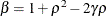where $\alpha = \gamma - \rho$ and $\beta = 1 + \rho ^2 - 2\gamma \rho$ . PROC HPLMIXED imposes the constraints $|\rho | < 1$ and $|\gamma | < 1$ for stationarity, although the resulting covariance matrix is not positive definite for some values of $\rho$ and $\gamma$ in this region. When the estimated value of $\rho$ becomes negative, the computed covariance is multiplied by $\cos (\pi d_{ij})$ to account for the negativity.

TYPE=CS

specifies the compound-symmetry structure, which has constant variance and constant covariance.

TYPE=CSH

specifies the heterogeneous compound-symmetry structure. This structure has a different variance parameter for each diagonal element, and it uses the square roots of these parameters in the off-diagonal entries. In Table 9.6, $\sigma ^2_ i$ is the i variance parameter, and $\rho$ is the correlation parameter that satisfies $|\rho | < 1$ .

TYPE=FA(q)

specifies the factor-analytic structure with q factors (Jennrich and Schluchter 1986). This structure is of the form $\bLambda \bLambda ’ + \bD$ , where $\bLambda$ is a $t \times q$ rectangular matrix and $\bD$ is a $t \times t$ diagonal matrix with t different parameters. When $\Argument{q} > 1$ , the elements of $\bLambda$ in its upper right corner (that is, the elements in the i row and j column for $j > i$ ) are set to zero to fix the rotation of the structure.

TYPE=FA0(q)

is similar to the FA(q) structure except that no diagonal matrix $\bD$ is included. When $\Argument{q} < t$ (that is, when the number of factors is less than the dimension of the matrix), this structure is nonnegative definite but not of full rank. In this situation, you can use this structure for approximating an unstructured $\bG$ matrix in the RANDOM statement. When $\Argument{q} = t$ , you can use this structure to constrain $\bG$ to be nonnegative definite in the RANDOM statement.

TYPE=FA1(q)

is similar to the TYPE=FA(q) structure except that all of the elements in $\bD$ are constrained to be equal. This offers a useful and more parsimonious alternative to the full factor-analytic structure.

TYPE=HF

specifies the Huynh-Feldt covariance structure (Huynh and Feldt 1970). This structure is similar to the TYPE=CSH structure in that it has the same number of parameters and heterogeneity along the main diagonal. However, it constructs the off-diagonal elements by taking arithmetic means rather than geometric means.

You can perform a likelihood ratio test of the Huynh-Feldt conditions by running PROC HPLMIXED twice, once with TYPE=HF and once with TYPE=UN , and then subtracting their respective values of $-2$ times the maximized likelihood.

If PROC HPLMIXED does not converge under your Huynh-Feldt model, you can specify your own starting values with the PARMS statement. The default MIVQUE(0) starting values can sometimes be poor for this structure. A good choice for starting values is often the parameter estimates that correspond to an initial fit that uses TYPE=CS .

TYPE=SIMPLE

is an alias for TYPE=VC .

TYPE=TOEP<(q)>

specifies a banded Toeplitz structure. This can be viewed as a moving average structure with order equal to $\Argument{q}-1$ . The TYPE=TOEP option is a full Toeplitz matrix, which can be viewed as an autoregressive structure with order equal to the dimension of the matrix. The specification TYPE=TOEP(1) is the same as $\sigma ^2 I$ , where I is an identity matrix, and it can be useful for specifying the same variance component for several effects.

TYPE=TOEPH<(q)>

specifies a heterogeneous banded Toeplitz structure. In Table 9.6, $\sigma ^2_ i$ is the i variance parameter and $\rho _ j$ is the j correlation parameter that satisfies $|\rho _ j| < 1$ . If you specify the order parameter q, then PROC HPLMIXED estimates only the first q bands of the matrix, setting all higher bands equal to 0. The option TOEPH(1) is equivalent to both the TYPE=UN (1) and TYPE=UNR (1) options.

TYPE=UN<(q)>

specifies a completely general (unstructured) covariance matrix that is parameterized directly in terms of variances and covariances. The variances are constrained to be nonnegative, and the covariances are unconstrained. This structure is not constrained to be nonnegative definite in order to avoid nonlinear constraints. However, you can use the TYPE=FA0 structure if you want this constraint to be imposed by a Cholesky factorization. If you specify the order parameter q, then PROC HPLMIXED estimates only the first q bands of the matrix, setting all higher bands equal to 0.

TYPE=UNR<(q)>

specifies a completely general (unstructured) covariance matrix that is parameterized in terms of variances and correlations. This structure fits the same model as the TYPE=UN (q) option but with a different parameterization. The i variance parameter is $\sigma ^2_ i$ . The parameter $\rho _{jk}$ is the correlation between the j and k measurements; it satisfies $|\rho _{jk}| < 1$ . If you specify the order parameter r, then PROC HPLMIXED estimates only the first q bands of the matrix, setting all higher bands equal to zero.

TYPE=VC

specifies standard variance components. This is the default structure for both the RANDOM and REPEATED statements. In the RANDOM statement, a distinct variance component is assigned to each effect.

Jennrich and Schluchter (1986) provide general information about the use of covariance structures, and Wolfinger (1996) presents details about many of the heterogeneous structures.