The HPLOGISTIC Procedure

- Performance Information
- Model Information
- Class Level Information
- Number of Observations
- Response Profile
- Selection Information
- Selection Summary
- Stop Reason
- Selection Reason
- Selected Effects
- Iteration History
- Convergence Status
- Dimensions
- Fit Statistics
- Global Tests
- Partition for the Hosmer and Lemeshow Test
- Hosmer and Lemeshow Goodness-of-Fit Test
- Association Statistics
- Parameter Estimates
The following sections describe the output that PROC HPLOGISTIC produces. The output is organized into various tables, which are discussed in the order of appearance.
The “Performance Information” table is produced by default. It displays information about the execution mode. For single-machine mode, the table displays the number of threads used. For distributed mode, the table displays the grid mode (symmetric or asymmetric), the number of compute nodes, and the number of threads per node.
If you specify the DETAILS option in the PERFORMANCE statement, the procedure also produces a “Timing” table in which elapsed time (absolute and relative) for the main tasks of the procedure are displayed.
The “Model Information” table displays basic information about the model, such as the response variable, frequency variable, link function, and the model category the HPLOGISTIC procedure determined based on your input and options. The “Model Information” table also displays the distribution of the data that is assumed by the HPLOGISTIC procedure. See the section Response Distributions for how the procedure determines the response distribution.
The “Class Level Information” table lists the levels of every variable specified in the CLASS statement. You should check this information to make sure that the data are correct. You can adjust the order of the CLASS variable levels with the ORDER= option in the CLASS statement. You can suppress the “Class Level Information” table completely or partially with the NOCLPRINT= option in the PROC HPLOGISTIC statement.
If the classification variables use reference parameterization, the “Class Level Information” table also displays the reference value for each variable.
The “Number of Observations” table displays the number of observations read from the input data set and the number of observations used in the analysis. If a FREQ statement is present, the sum of the frequencies read and used is displayed. If the events/trials syntax is used, the number of events and trials is also displayed.
The “Response Profile” table displays the ordered value from which the HPLOGISTIC procedure determines the probability being modeled as an event in binary models and the ordering of categories in multinomial models. For each response category level, the frequency used in the analysis is reported. You can affect the ordering of the response values with the response-options in the MODEL statement. For binary and generalized logit models, the note that follows the “Response Profile” table indicates which outcome is modeled as the event in binary models and which value serves as the reference category.
The “Response Profile” table is not produced for binomial data. You can find information about the number of events and trials in the “Number of Observations” table.
When you specify the SELECTION statement, the HPLOGISTIC procedure produces by default a series of tables with information about the model selection. The “Selection Information” table informs you about the model selection method, selection and stop criteria, and other parameters that govern the selection. You can suppress this table by specifying DETAILS=NONE in the SELECTION statement.
When you specify the SELECTION statement, the HPLOGISTIC procedure produces the “Selection Summary” table with information about which effects were entered into or removed from the model at the steps of the model selection process. The p-value for the score chi-square test that led to the removal or entry decision is also displayed. You can request further details about the model selection steps by specifying DETAILS=STEPS or DETAILS=ALL in the SELECTION statement. You can suppress the display of the “Selection Summary” table by specifying DETAILS=NONE in the SELECTION statement.
When you specify the SELECTION statement, the HPLOGISTIC procedure produces a simple table that tells you why model selection stopped.
When you specify the SELECTION statement, the HPLOGISTIC procedure produces a simple table that tells you why the final model was selected.
When you specify the SELECTION statement, the HPLOGISTIC procedure produces a simple table that tells you which effects were selected into the final model.
For each iteration of the optimization, the “Iteration History” table displays the number of function evaluations (including gradient and Hessian evaluations), the value of the objective function, the change in the objective function from the previous iteration and the absolute value of the largest (projected) gradient element. The objective function used in the optimization in the HPLOGISTIC procedure is normalized by default to enable comparisons across data sets with different sampling intensity. You can control normalization with the NORMALIZE= option in the PROC HPLOGISTIC statement.
If you specify the ITDETAILS option in the PROC HPLOGISTIC statement, information about the parameter estimates and gradients in the course of the optimization is added to the “Iteration History” table.
The “Iteration History” table is displayed by default unless you specify the NOITPRINT option or perform a model selection. To generate the history from a model selection process, specify the ITSELECT option.
The convergence status table is a small ODS table that follows the “Iteration History” table in the default output. In the listing it appears as a message that indicates whether the optimization succeeded and
which convergence criterion was met. If the optimization fails, the message indicates the reason for the failure. If you save
the convergence status table to an output data set, a numeric Status variable is added that enables you to assess convergence programmatically. The values of the Status variable encode the following:
- 0
-
Convergence was achieved, or an optimization was not performed (because TECHNIQUE=NONE is specified).
- 1
-
The objective function could not be improved.
- 2
-
Convergence was not achieved because of a user interrupt or because a limit was exceeded, such as the maximum number of iterations or the maximum number of function evaluations. To modify these limits, see the MAXITER=, MAXFUNC=, and MAXTIME= options in the PROC HPLOGISTIC statement.
- 3
-
Optimization failed to converge because function or derivative evaluations failed at the starting values or during the iterations or because a feasible point that satisfies the parameter constraints could not be found in the parameter space.
The “Dimensions” table displays size measures that are derived from the model and the environment. For example, it displays the number of columns in the design matrix, the rank of the matrix, the largest number of design columns associated with an effect, the number of compute nodes in distributed mode, and the number of threads per node.
The “Fit Statistics” table displays a variety of likelihood-based measures of fit. All statistics are presented in “smaller is better” form.
The calculation of the information criteria uses the following formulas, where ![]() denotes the number of effective parameters,
denotes the number of effective parameters, ![]() denotes the number of frequencies used, and
denotes the number of frequencies used, and ![]() is the log likelihood evaluated at the converged estimates:
is the log likelihood evaluated at the converged estimates:
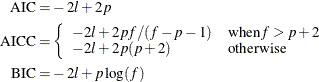
If no FREQ statement is given, ![]() equals
equals ![]() , the number of observations used.
, the number of observations used.
The values displayed in the “Fit Statistics” table are not based on a normalized log-likelihood function.
The “Global Tests” table provides a statistical test for the hypothesis of whether the final model provides a better fit than a model without effects (an “intercept-only” model).
If you specify the NOINT option in the MODEL statement, the reference model is one where the linear predictor is 0 for all observations.
The “Partition for the Hosmer and Lemeshow Test” table displays the grouping used in the Hosmer-Lemeshow test. This table is displayed if you specify the LACKFIT option in the MODEL statement. See the section The Hosmer-Lemeshow Goodness-of-Fit Test for details, and see Hosmer and Lemeshow (2000) for examples of using this partition.
The “Hosmer and Lemeshow Goodness-of-Fit Test” table provides a test of the fit of the model; small p-values reject the null hypothesis that the fitted model is adequate. This table is displayed if you specify the LACKFIT option in the MODEL statement. See the section The Hosmer-Lemeshow Goodness-of-Fit Test for further details.
The “Association Statistics” table displays the concordance index C (the area under the ROC curve, AUC), Somers’ D statistic (Gini’s coefficient), Goodman-Kruskal’s gamma statistic, and Kendall’s tau-a statistic. This table is displayed if you specify the ASSOCIATION option in the MODEL statement.
The parameter estimates, their estimated (asymptotic) standard errors, and p-values for the hypothesis that the parameter is 0 are presented in the “Parameter Estimates” table. If you request confidence intervals with the CL or ALPHA= options in the MODEL statement, confidence limits are produced for the estimate on the linear scale.