The HPLOGISTIC Procedure

The HPLOGISTIC procedure forms the log-likelihood functions of the various models as
where ![]() is the log-likelihood contribution of the
is the log-likelihood contribution of the ![]() th observation with weight
th observation with weight ![]() and
and ![]() is the value of the frequency variable. For the determination of
is the value of the frequency variable. For the determination of ![]() and
and ![]() , see the WEIGHT and FREQ statements. The individual log-likelihood contributions for the various distributions are as follows.
, see the WEIGHT and FREQ statements. The individual log-likelihood contributions for the various distributions are as follows.
The HPLOGISTIC procedure computes the log-likelihood function ![]() for the
for the ![]() th binary observation as
th binary observation as
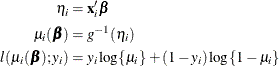
Here, ![]() is the probability of an event, and the variable
is the probability of an event, and the variable ![]() takes on the value 1 for an event and the value 0 for a non-event. The inverse link function
takes on the value 1 for an event and the value 0 for a non-event. The inverse link function ![]() maps from the scale of the linear predictor
maps from the scale of the linear predictor ![]() to the scale of the mean. For example, for the logit link (the default),
to the scale of the mean. For example, for the logit link (the default),
You can control which binary outcome in your data is modeled as the event with the response-options in the MODEL statement, and you can choose the link function with the LINK= option in the MODEL statement.
If a WEIGHT statement is given and ![]() denotes the weight for the current observation, the log-likelihood function is computed as
denotes the weight for the current observation, the log-likelihood function is computed as
The HPLOGISTIC procedure computes the log-likelihood function ![]() for the
for the ![]() th binomial observation as
th binomial observation as
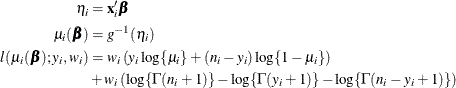
where ![]() and
and ![]() are the values of the events and trials of the
are the values of the events and trials of the ![]() th observation, respectively.
th observation, respectively. ![]() measures the probability of events (successes) in the underlying Bernoulli distribution whose aggregate follows the binomial
distribution.
measures the probability of events (successes) in the underlying Bernoulli distribution whose aggregate follows the binomial
distribution.
The multinomial distribution modeled by the HPLOGISTIC procedure is a generalization of the binary distribution; it is the
distribution of a single draw from a discrete distribution with ![]() possible values. The log-likelihood function for the
possible values. The log-likelihood function for the ![]() th observation is thus deceptively simple:
th observation is thus deceptively simple:
In this expression, ![]() denotes the number of response categories (the number of possible outcomes) and
denotes the number of response categories (the number of possible outcomes) and ![]() is the probability that the
is the probability that the ![]() th observation takes on the response value associated with category
th observation takes on the response value associated with category ![]() . The category probabilities must satisfy
. The category probabilities must satisfy
and the constraint is satisfied by modeling ![]() categories. In models with ordered response categories, the probabilities are expressed in cumulative form, so that the last
category is redundant. In generalized logit models (multinomial models with unordered categories), one category is chosen
as the reference category and the linear predictor in the reference category is set to zero.
categories. In models with ordered response categories, the probabilities are expressed in cumulative form, so that the last
category is redundant. In generalized logit models (multinomial models with unordered categories), one category is chosen
as the reference category and the linear predictor in the reference category is set to zero.