| Calculating Principal Components |
Principal Component Plots
Examine the scatter plot of the first two principal components shown in Figure 19.6. Each marker on the plot represents two principal component scores. The output component scores are a linear combination of the standardized Y variables with coefficients equal to the eigenvectors of the correlation matrix.
| Click on the observations with the four highest values for PCR1. |
The resulting scatter plot should now appear as shown in Figure 19.8.
These four observations correspond to Mike Schmidt, Reggie Jackson, Tony Perez, and Pete Rose. The label for Mike Schmidt is not shown because the observation is too close to Reggie Jackson. This is not unexpected since the first principal component is a measure of the player's overall career performance.
Now examine observations in the second principal component direction on the scatter plot. Recall that the second component appeared to be a measure of the combined performance of home runs and runs batted in versus other career performance. The observations with large values of PCR2 correspond to Mike Schmidt and Reggie Jackson. As one might expect, both players have high career-long home runs and runs batted in.
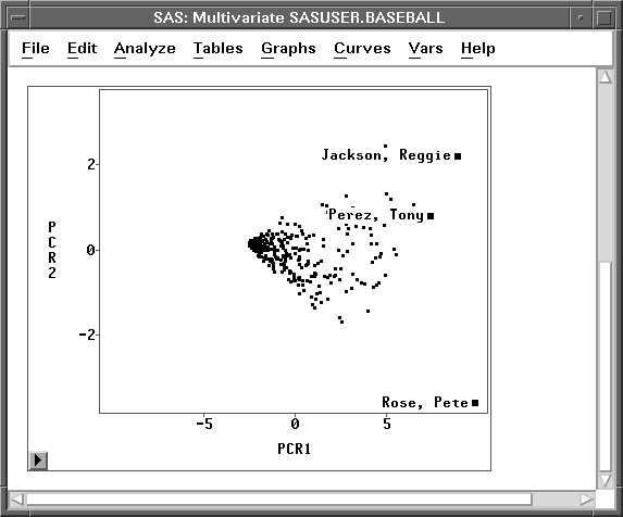
Figure 19.8: Scatter Plot of First Two Principal Components
Copyright © 2007 by SAS Institute Inc., Cary, NC, USA. All rights reserved.