Calculating Principal Components

Calculating Principal Components

Principal component analysis summarizes high dimensional data into a few dimensions. Each dimension is called a principal component and represents a linear combination of the variables. The first principal component accounts for as much variation in the data as possible. Each succeeding principal component accounts for as much of the variation unaccounted for by preceding principal components as possible.

Consider the BASEBALL data set. These data contain performance measures and salary levels for regular hitters and leading substitute hitters in the major leagues in 1986. Suppose you are interested in exploring the relationship between players' performances and their salaries.

If you can first reduce the six career hitting and fielding variables into two or three dimensions -that is, two or three linear combinations of these variables -then graphing these against the SALARY variable would be useful. You can then look for relationships between performance and salary.

To create the principal component analysis, follow these steps.

Open the BASEBALL data set.

Choose Analyze:Multivariate (Y's).

[menu]
Figure 19.2: Analyze Menu

Select the fifteen hitting and fielding variables in the list at the left.

These are CR_ATBAT, CR_HITS, CR_HOME, CR_RUNS, CR_RBI, and CR_BB. Then Click the Y button. The selected variables appear in the Y variables list.

Select NAME in the list at the left, then click the Label button.

NAME appears in the Label variables list. Your variables dialog should now appear as shown in Figure 19.3.

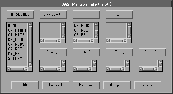
Figure 19.3: Variables Dialog with Variable Roles Assigned

Click the Output button.

The output options dialog appears.

Click the Principal Component Analysis check box in the output options dialog

This requests a principal component analysis. Your output options dialog should now appear as shown in Figure 19.4.

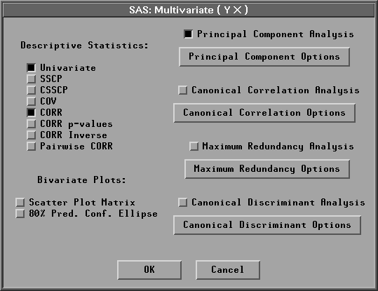
Figure 19.4: Multivariate Output Options Dialog

Click the Principal Component Options button in the output options dialog

A principal component options dialog should now appear as shown in Figure 19.5.

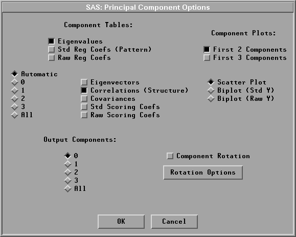
Figure 19.5: Principal Component Options Dialog

Click the Eigenvectors check box in the principal component options dialog

Click the radio mark 2 in the options dialog

This requests that the first two principal components are used for tables of eigenvectors and correlations.

Note	By default, the analysis is carried out on the correlation matrix. You can use the covariance matrix instead by setting options with the Method button in the Multivariate variables dialog. The covariance matrix is recommended only when all the variables are measured in comparable units.

Click OK in all dialogs.

A multivariate window appears. At the bottom of the window is the principal component analysis, as shown in Figure 19.6.

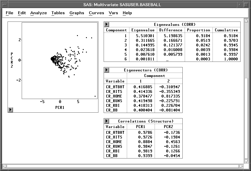
Figure 19.6: Multivariate Window

Principal Component Tables

Principal Component Plots

Top of Page