The RELIABILITY Procedure
- Overview
-
Getting Started
 Analysis of Right-Censored Data from a Single PopulationWeibull Analysis Comparing Groups of DataAnalysis of Accelerated Life Test DataWeibull Analysis of Interval Data with Common Inspection ScheduleLognormal Analysis with Arbitrary CensoringRegression ModelingRegression Model with Nonconstant ScaleRegression Model with Two Independent VariablesWeibull Probability Plot for Two Combined Failure ModesAnalysis of Recurrence Data on RepairsComparison of Two Samples of Repair DataAnalysis of Interval Age Recurrence DataAnalysis of Binomial DataThree-Parameter WeibullParametric Model for Recurrent Events DataParametric Model for Interval Recurrent Events Data
 -
SyntaxPrimary StatementsSecondary StatementsGraphical Enhancement StatementsPROC RELIABILITY StatementANALYZE StatementBY StatementCLASS StatementDISTRIBUTION StatementEFFECTPLOT StatementESTIMATE StatementFMODE StatementFREQ StatementINSET StatementLOGSCALE StatementLSMEANS StatementLSMESTIMATE StatementMAKE StatementMCFPLOT StatementMODEL StatementNENTER StatementNLOPTIONS StatementPROBPLOT StatementRELATIONPLOT StatementSLICE StatementSTORE StatementTEST StatementUNITID Statement
-
DetailsAbbreviations and NotationTypes of Lifetime DataProbability DistributionsProbability PlottingNonparametric Confidence Intervals for Cumulative Failure ProbabilitiesParameter Estimation and Confidence IntervalsRegression Model Statistics Computed for Each Observation for Lifetime DataRegression Model Statistics Computed for Each Observation for Recurrent Events DataRecurrence Data from Repairable SystemsODS Table NamesODS Graphics
- References
This example illustrates analyzing data that have more general censoring than in the previous example. The data can be a combination of exact failure times, left censored, right censored, and interval censored data. The intervals can be overlapping, unlike in the previous example, where the interval endpoints had to be the same for all units.
Table 16.2 shows data from Nelson (1982, p. 409), analyzed by Meeker and Escobar (1998, p. 135). Each of 435 turbine wheels was inspected once to determine whether a crack had developed in the wheel or not. The inspection time (in 100s of hours), the number inspected at the time that had cracked, and the number not cracked are shown in the table. The quantity of interest is the time for a crack to develop.
Table 16.2: Turbine Wheel Cracking Data
|
Inspection Time |
Number |
Number |
|---|---|---|
|
(100 hours) |
Cracked |
Not Cracked |
|
4 |
0 |
39 |
|
10 |
4 |
49 |
|
14 |
2 |
31 |
|
18 |
7 |
66 |
|
22 |
5 |
25 |
|
26 |
9 |
30 |
|
30 |
9 |
33 |
|
34 |
6 |
7 |
|
38 |
22 |
12 |
|
42 |
21 |
19 |
|
46 |
21 |
15 |
These data consist only of left and right censored lifetimes. If a unit exhibits a crack at an inspection time, the unit is left censored at the time; if a unit has not developed a crack, it is right censored at the time. For example, there are 4 left-censored lifetimes and 49 right-censored lifetimes at 1000 hours.
The following statements create a SAS data set named TURBINE that contains the data in the format necessary for analysis by the RELIABILITY procedure:
data turbine;
   label t1 = 'Time of Cracking (Hours x 100 )';
   input t1 t2 f;
   datalines;
.   4  0
4   .  39
.  10  4
10  .  49
.  14  2
14  .  31
.  18  7
18  .  66
.  22  5
22  .  25
.  26  9
26  .  30
.  30  9
30  .  33
.  34  6
34  .  7
.  38  22
38  .  12
.  42  21
42  .  19
.  46  21
46  .  15
;
The variables T1 and T2 represent the inspection times and determine whether the observation is right or left censored. If T1 is missing (.), then T2 represents a left-censoring time; if T2 is missing, T1 represents a right-censoring time. The variable F is the number of units that were found to be cracked for left-censored observations, or not cracked for right-censored observations
at an inspection time.
The following statements use the RELIABILITY procedure to produce the probability plot in Figure 16.15 for the data in the data set TURBINE:
proc reliability data = turbine;
   distribution lognormal;
   freq f;
   pplot ( t1 t2 ) / maxitem = 5000
                     ppout;
run;
The DISTRIBUTION statement specifies that a lognormal probability plot be created. The FREQ statement identifies the frequency
variable F. The option MAXITEM=5000 specifies that the iterative algorithm that computes the points on the probability plot takes a
maximum of 5000 iterations. The algorithm does not converge for these data in the default 1000 iterations, so the maximum
number of iterations needs to be increased for convergence. The option PPOUT specifies that a table of the cumulative probabilities
plotted on the probability plot be printed, along with standard errors and confidence limits.
The tabular output for the maximum likelihood lognormal fit for these data is shown in Figure 16.16. Figure 16.15 shows the resulting lognormal probability plot with the computed cumulative probability estimates and the lognormal fit line.
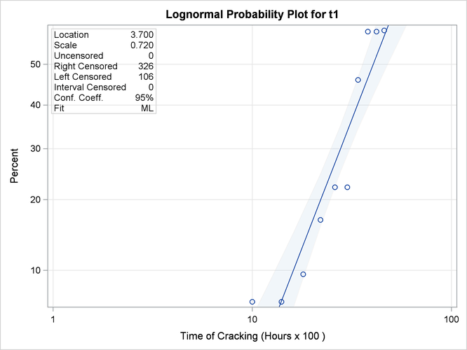
Figure 16.16: Partial Listing of the Tabular Output for the Turbine Wheel Data
| Cumulative Probability Estimates | |||||
|---|---|---|---|---|---|
| Lower Lifetime | Upper Lifetime | Cumulative Probability |
Pointwise 95% Confidence Limits |
Standard Error |
|
| Lower | Upper | ||||
| . | 4 | 0.0000 | 0.0000 | 0.0000 | 0.0000 |
| 10 | 10 | 0.0698 | 0.0264 | 0.1720 | 0.0337 |
| 14 | 14 | 0.0698 | 0.0177 | 0.2384 | 0.0473 |
| 18 | 18 | 0.0959 | 0.0464 | 0.1878 | 0.0345 |
| 22 | 22 | 0.1667 | 0.0711 | 0.3432 | 0.0680 |
| 26 | 26 | 0.2222 | 0.1195 | 0.3757 | 0.0657 |
| 30 | 30 | 0.2222 | 0.1203 | 0.3738 | 0.0650 |
| 34 | 34 | 0.4615 | 0.2236 | 0.7184 | 0.1383 |
| 38 | 38 | 0.5809 | 0.4085 | 0.7356 | 0.0865 |
| 42 | 42 | 0.5809 | 0.4280 | 0.7198 | 0.0766 |
| 46 | 46 | 0.5836 | 0.4195 | 0.7311 | 0.0822 |