The RELIABILITY Procedure
- Overview
-
Getting Started
 Analysis of Right-Censored Data from a Single PopulationWeibull Analysis Comparing Groups of DataAnalysis of Accelerated Life Test DataWeibull Analysis of Interval Data with Common Inspection ScheduleLognormal Analysis with Arbitrary CensoringRegression ModelingRegression Model with Nonconstant ScaleRegression Model with Two Independent VariablesWeibull Probability Plot for Two Combined Failure ModesAnalysis of Recurrence Data on RepairsComparison of Two Samples of Repair DataAnalysis of Interval Age Recurrence DataAnalysis of Binomial DataThree-Parameter WeibullParametric Model for Recurrent Events DataParametric Model for Interval Recurrent Events Data
 -
SyntaxPrimary StatementsSecondary StatementsGraphical Enhancement StatementsPROC RELIABILITY StatementANALYZE StatementBY StatementCLASS StatementDISTRIBUTION StatementEFFECTPLOT StatementESTIMATE StatementFMODE StatementFREQ StatementINSET StatementLOGSCALE StatementLSMEANS StatementLSMESTIMATE StatementMAKE StatementMCFPLOT StatementMODEL StatementNENTER StatementNLOPTIONS StatementPROBPLOT StatementRELATIONPLOT StatementSLICE StatementSTORE StatementTEST StatementUNITID Statement
-
DetailsAbbreviations and NotationTypes of Lifetime DataProbability DistributionsProbability PlottingNonparametric Confidence Intervals for Cumulative Failure ProbabilitiesParameter Estimation and Confidence IntervalsRegression Model Statistics Computed for Each Observation for Lifetime DataRegression Model Statistics Computed for Each Observation for Recurrent Events DataRecurrence Data from Repairable SystemsODS Table NamesODS Graphics
- References
The following example illustrates the analysis of an accelerated life test for Class B electrical motor insulation. The data
are provided by Nelson (1990, p. 243). Forty insulation specimens were tested at four temperatures: ![]() ,
, ![]() ,
, ![]() , and
, and ![]() C. The purpose of the test is to estimate the median life of the insulation at the design operating temperature of
C. The purpose of the test is to estimate the median life of the insulation at the design operating temperature of ![]() C.
C.
The following SAS program creates the data listed in Figure 16.8. Ten specimens of the insulation were tested at each test temperature. The variable Time provides a specimen time to failure or a censoring time, in hours. The variable Censor is equal to 1 if the value of the variable Time is a right-censoring time and is equal to 0 if the value is a failure time. Some censor times and failure times are identical
at some of the temperatures. Rather than repeating identical observations in the input data set, the variable Count provides the number of specimens with identical times and temperatures. The variable Temp provides the test temperature in degrees centigrade. The variable Cntrsl is a control variable specifying that percentiles are to be computed only for the first value of Temp (![]() C). The value of
C). The value of Temp in the first observation (![]() C) does not correspond to a test temperature. The missing values in the first observation cause the observation to be excluded
from the model fit, and the value of 1 for the variable
C) does not correspond to a test temperature. The missing values in the first observation cause the observation to be excluded
from the model fit, and the value of 1 for the variable Cntrl causes percentiles corresponding to a temperature of ![]() C to be computed.
C to be computed.
data classb;
   input hours temp count censor;
   if _n_ = 1 then cntrl=1;
   else cntrl=0;
   label hours='Hours';
   datalines;
   . 130 .  .
8064 150 10 1
1764 170 1  0
2772 170 1  0
3444 170 1  0
3542 170 1  0
3780 170 1  0
4860 170 1  0
5196 170 1  0
5448 170 3  1
 408 190 2  0
1344 190 2  0
1440 190 1  0
1680 190 5  1
 408 220 2  0
 504 220 3  0
 528 220 5  1
;
Figure 16.8: Listing of the Class B Insulation Data
| Obs | hours | temp | count | censor | cntrl |
|---|---|---|---|---|---|
| 1 | . | 130 | . | . | 1 |
| 2 | 8064 | 150 | 10 | 1 | 0 |
| 3 | 1764 | 170 | 1 | 0 | 0 |
| 4 | 2772 | 170 | 1 | 0 | 0 |
| 5 | 3444 | 170 | 1 | 0 | 0 |
| 6 | 3542 | 170 | 1 | 0 | 0 |
| 7 | 3780 | 170 | 1 | 0 | 0 |
| 8 | 4860 | 170 | 1 | 0 | 0 |
| 9 | 5196 | 170 | 1 | 0 | 0 |
| 10 | 5448 | 170 | 3 | 1 | 0 |
| 11 | 408 | 190 | 2 | 0 | 0 |
| 12 | 1344 | 190 | 2 | 0 | 0 |
| 13 | 1440 | 190 | 1 | 0 | 0 |
| 14 | 1680 | 190 | 5 | 1 | 0 |
| 15 | 408 | 220 | 2 | 0 | 0 |
| 16 | 504 | 220 | 3 | 0 | 0 |
| 17 | 528 | 220 | 5 | 1 | 0 |
An Arrhenius-lognormal model is fitted to the data in this example. In other words, the failure times follow a lognormal (base
10) distribution, and the lognormal location parameter ![]() depends on the centigrade temperature
depends on the centigrade temperature Temp through the Arrhenius relationship
where
is 1000 times the reciprocal absolute temperature. The lognormal (base e) distribution is also available.
The following SAS statements fit the Arrhenius-lognormal model, and they display the fitted model distributions side-by-side on the probability and the relation plots shown in Figure 16.9:
proc reliability;
   distribution lognormal10;
   freq count;
   model hours*censor(1) = temp /
      relation = arr
      obstats(quantile = .1 .5 .9 control = cntrl);
   rplot hours*censor(1) = temp /
      pplot
      fit = model
      noconf
      relation = arr
      plotdata
      plotfit 10 50 90
      lupper = 1.e5
      slower = 120;
run;
The PROC RELIABILITY statement invokes the procedure and specifies CLASSB as the input data set. The DISTRIBUTION statement specifies that the lognormal (base 10) distribution is to be used for maximum
likelihood parameter estimation and probability plotting. The FREQ statement specifies that the variable Count is to be used as a frequency variable; that is, if Count=n, then there are n specimens with the time and temperature specified in the observation.
The MODEL statement fits a linear regression equation for the distribution location parameter as a function of independent
variables. In this case, the MODEL statement also transforms the independent variable through the Arrhenius relationship.
The dependent variable is specified as Time. A value of 1 for the variable Censor indicates that the corresponding value of Time is a right-censored observation; otherwise, the value is a failure time. The temperature variable Temp is specified as the independent variable in the model. The MODEL statement option RELATION=ARR specifies the Arrhenius relationship.
The option OBSTATS requests statistics computed for each observation in the input data set. The options in parentheses following
OBSTATS indicate which statistics are to be computed. In this case, QUANTILE=.1 .5 .9 specifies that quantiles of the fitted
distribution are to be computed for the value of the variable Temp at each observation. The CONTROL= option requests quantiles only for those observations in which the variable Cntrl has a value of 1. This eliminates unnecessary quantiles in the OBSTATS table since, in this case, only the quantiles at the
design temperature of ![]() C are of interest.
C are of interest.
The RPLOT, or RELATIONPLOT, statement displays a plot of the lifetime data and the fitted model. The dependent variable Time, the independent variable Temp, and the censoring indicator Censor are the same as in the MODEL statement. The option FIT=MODEL specifies that the model fitted with the preceding MODEL statement
is to be used for probability plotting and in the relation plot. The option RELATION=ARR specifies an Arrhenius scale for
the horizontal axis of the relation plot. The PPLOT option specifies that a probability plot is to be displayed alongside
the relation plot. The type of probability plot is determined by the distribution named in the DISTRIBUTION statement, in
this case, a lognormal (base 10) distribution. Weibull, extreme value, lognormal (base e), normal, log-logistic, and logistic distributions are also available. The NOCONF option suppresses the default percentile
confidence bands on the probability plot. The PLOTDATA option specifies that the failure times are to be plotted on the relation
plot. The PLOTFIT option specifies that the 10th, 50th, and 90th percentiles of the fitted relationship are to be plotted
on the relation plot. The options LUPPER and SLOWER specify an upper limit on the life axis scale and a lower limit on the
stress (temperature) axis scale in the plots.
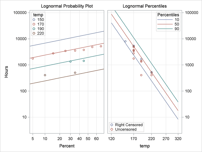
The plots produced by the preceding statements are shown in Figure 16.9. The plot on the left is an overlaid lognormal probability plot of the data and the fitted model. The plot on the right is a relation plot showing the data and the fitted relation. The fitted straight lines are percentiles of the fitted distribution at each temperature. An Arrhenius relation fitted to the data, plotted on an Arrhenius plot, yields straight percentile lines.
Since all the data at ![]() C are right censored, there are no failures corresponding to
C are right censored, there are no failures corresponding to ![]() C on the probability plot. However, the fitted distribution at
C on the probability plot. However, the fitted distribution at ![]() C is plotted on the probability plot.
C is plotted on the probability plot.
The tabular output requested with the MODEL statement is shown in Figure 16.10. The "Model Information" table provides general information about the data and model. The "Summary of Fit" table shows the number of observations used, the number of failures and of censored values (accounting for the frequency count), and the maximum log likelihood for the fitted model.
The "Lognormal Parameter Estimates" table contains the Arrhenius-lognormal model parameter estimates, their standard errors,
and confidence interval estimates. In this table, INTERCEPT is the maximum likelihood estimate of ![]() , TEMP is the estimate of
, TEMP is the estimate of ![]() , and Scale is the estimate of the lognormal scale parameter,
, and Scale is the estimate of the lognormal scale parameter, ![]() .
.
The "Observation Statistics" table provides the estimates of the fitted distribution quantiles, their standard errors, and
the confidence limits. These are given only for the value of ![]() C, as specified with the CONTROL= option in the MODEL statement. The predicted median life at
C, as specified with the CONTROL= option in the MODEL statement. The predicted median life at ![]() C corresponds to a quantile of 0.5, and it is approximately 47,135 hours.
C corresponds to a quantile of 0.5, and it is approximately 47,135 hours.
In addition to the MODEL statement output in Figure 16.10, the RELIABILITY procedure produces tabular output for each temperature that is identical to the output produced with the PROBPLOT statement. This output is not shown.