The RELIABILITY Procedure

Weibull Probability Plot for Two Combined Failure Modes

Doganaksoy, Hahn, and Meeker (2002) analyzed failure data for the dielectric insulation of generator armature bars. A sample of 58 segments of bars were subjected to a high voltage stress test. Based on examination of the sample after the test, failures were attributed to one of two modes:

Mode D (degradation failure): degradation of the organic material. Such failures usually occur later in life.
Mode E (early failure): insulation defects due to a processing problem. These failures tend to occur early in life.

The following SAS statements create a SAS data set that contains the failure data:

data Voltage;
   input Hours Mode$ @@;
   if Mode = 'Cen' then Status = 1;
   else Status = 0;
   datalines;
2   E   3   E   5   E   8   E   13  Cen 21  E
28  E   31  E   31  Cen 52  Cen 53  Cen 64  E
67  Cen 69  E   76  E   78  Cen 104 E   113 Cen
119 E   135 Cen 144 E   157 Cen 160 E   168 D
179 Cen 191 D   203 D   211 D   221 E   226 D
236 E   241 Cen 257 Cen 261 D   264 D   278 D
282 E   284 D   286 D   298 D   303 E   314 D
317 D   318 D   320 D   327 D   328 D   328 D
348 D   348 Cen 350 D   360 D   369 D   377 D
387 D   392 D   412 D   446 D
;

The variable Hours represents the number of hours until a failure, or the number of hours on test if the sample unit did not fail. The variable Mode represents the failure mode: D for degradation failure, E for early failures, or Cen if the unit did not fail (i.e., is right-censored). The computed variable Status is a numeric indicator for censored observations.

The following statements fit a Weibull distribution to the individual failure modes (D and E), and compute the failure distribution with both modes acting:

proc reliability data=Voltage;
   distribution Weibull;
   pplot Hours*Status(1) / vref(intersect) = 10  
                           vreflabel = ('10% Percentile')
                           survtime = 100 200 300 400 500 1000
                           lupper = 500;
   fmode combine = Mode( 'D' 'E' );
run;

Figure 16.27 contains estimates of the combined failure mode survival function at the times specified with the SURVTIME= option in the PPLOT statement.

Figure 16.27: Survival Function Estimates for Combined Failure Modes

The RELIABILITY Procedure

Combined Failure Modes
Weibull Distribution Function Estimates
With 95% Asymptotic Normal Confidence Limits
X	Pr(<X)	Lower	Upper	Pr(>X)	Lower	Upper
100.00	0.1898	0.1172	0.2926	0.8102	0.7074	0.8828
200.00	0.3115	0.2139	0.4292	0.6885	0.5708	0.7861
300.00	0.5866	0.4621	0.7010	0.4134	0.2990	0.5379
400.00	0.9405	0.8476	0.9782	0.0595	0.0218	0.1524
500.00	0.9998	0.9711	1.0000	0.0002	0.0000	0.0289
1000.00	1.0000	0.0000	1.0000	0.0000	0.0000	1.0000

Figure 16.28 shows Weibull parameter estimates for the two individual failure modes.

Figure 16.28: Parameter Estimates for Individual Failure Modes

Individual Failure Mode
Weibull Parameter Estimates
Parameter	Estimate	Standard Error	Asymptotic Normal		Mode
			95% Confidence Limits
			Lower	Upper
EV Location	5.8415	0.0350	5.7730	5.9100	D
EV Scale	0.1785	0.0254	0.1350	0.2360	D
Weibull Scale	344.2966	12.0394	321.4903	368.7208	D
Weibull Shape	5.6020	0.7985	4.2365	7.4076	D

EV Location	7.0649	0.5109	6.0637	8.0662	E
EV Scale	1.5739	0.3415	1.0287	2.4080	E
Weibull Scale	1170.1832	597.7903	429.9480	3184.8703	E
Weibull Shape	0.6354	0.1379	0.4153	0.9721	E

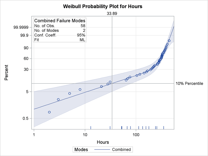
Figure 16.29 is a Weibull probability plot of the failure probability distribution with the two failure modes combined, along with approximate pointwise 95% confidence limits. A reference line at the 10% point on the vertical axis intersecting the distribution curve shows the 10% percentile of lifetimes when both modes act to be about 34 hours.

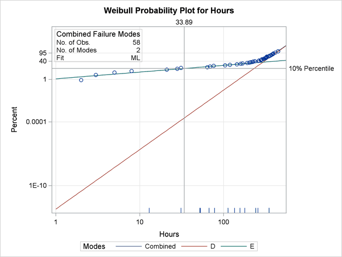
Figure 16.29: Weibull Plot for Failure Modes D and E

The following SAS statements create the Weibull probability plot in Figure 16.30:

proc reliability data=Voltage;
   distribution Weibull;
   pplot Hours*Status(1) / vref(intersect) = 10  
                           vreflabel = ('10% Percentile')
                           survtime = 100 200 300 400 500 1000
                           noconf
                           lupper = 500;
   fmode combine = Mode( 'D' 'E' ) / plotmodes;
run;

The PLOTMODES option in the FMODE statement cause the Weibull fits for the individual failure modes to be included on the probability plot. The combined failure mode curve is almost the same as the fit curve for mode E for lifetimes less than 100 hours, and slightly greater than the fit curve for mode D for lifetimes greater than 100 hours.

Figure 16.30: Weibull Plot for Failure Modes D and E with Individual Modes