PROC RELIABILITY: Recurrence Data from Repairable Systems

Recurrence Data from Repairable Systems

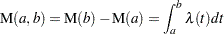
Failures in a system that can be repaired are sometimes modeled as recurrence data, or recurrent events data. When a repairable system fails, it is repaired and placed back in service. As a repairable system ages, it accumulates a history of repairs and costs of repairs. The mean cumulative function (MCF) $\text{[math]}$ is defined as the population mean of the cumulative number (or cost) of repairs up until time $\text{[math]}$ . You can use the RELIABILITY procedure to compute and plot nonparametric estimates and plots of the MCF for the number of repairs or the cost of repairs. The Nelson (1995) confidence limits for the MCF are also computed and plotted. You can compute and plot estimates of the difference of two MCFs and confidence intervals. This is useful for comparing the repair performance of two systems.

See Nelson (2002, 1995, 1988) , Doganaksoy and Nelson (1998) , and Nelson and Doganaksoy (1989) for discussions and examples of nonparametric analysis of recurrence data.

You can also fit a parametric model for recurrent event data and display the resulting model on a plot, along with nonparametric estimates of the MCF.

See Rigdon and Basu (2000), Tobias and Trindade (1995), and Meeker and Escobar (1998) for discussions of parametric models for recurrent events data.

Nonparametric Analysis

Recurrent Events Data with Exact Ages

See the section Analysis of Recurrence Data on Repairs and the section Comparison of Two Samples of Repair Data for examples of the analysis of recurrence data with exact ages.

Formulas for the MCF estimator $\text{[math]}$ and the variance of the estimator Var $\text{[math]}$ are given in Nelson (1995). Table 14.64 shows a set of artificial repair data from Nelson (1988). For each system, the data consist of the system and cost for each repair. If you want to compute the MCF for the number of repairs, rather than cost of repairs, then you should set the cost equal to 1 for each repair. A plus sign (+) in place of a cost indicates that the age is a censoring time. The repair history of each system ends with a censoring time.

Table 14.64 System Repair Histories for Artificial Data
Unit	(Age in Months, Cost in $100)
6	(5,$3)	(12,$1)	(12,+)
5	(16,+)
4	(2,$1)	(8,$1)	(16,$2)	(20,+)
3	(18,$3)	(29,+)
2	(8,$2)	(14,$1)	(26,$1)	(33,+)
1	(19,$2)	(39,$2)	(42,+)

Table 14.65 illustrates the calculation of the MCF estimate from the data in Table 14.64. The RELIABILITY procedure uses the following rules for computing the MCF estimates.

Order all events (repairs and censoring) by age from smallest to largest.
- If the event ages of the same or different systems are equal, the corresponding data are sorted from the largest repair cost to the smallest. Censoring events always sort as smaller than repair events with equal ages.
- When event ages and values of more than one system coincide, the corresponding data are sorted from the largest system identifier to the smallest. The system IDs can be numeric or character, but they are always sorted in ASCII order.
Compute the number of systems $\text{[math]}$ in service at the current age as the number in service at the last repair time minus the number of censored units in the intervening times.
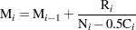
For each repair, compute the mean cost as the cost of the current repair divided by the number in service $\text{[math]}$ .
Compute the MCF for each repair as the previous MCF plus the mean cost for the current repair.

Table 14.65 Calculation of MCF for Artificial Data
Event	(Age,Cost)	Service	Cost	MCF
		Number $\text{[math]}$ in	Mean
1	(2,$1)	6	$1/6=0.17	0.17
2	(5,$3)	6	$3/6=0.50	0.67
3	(8,$2)	6	$2/6=0.33	1.00
4	(8,$1)	6	$1/6=0.17	1.17
5	(12,$1)	6	$1/6=0.17	1.33
6	(12,+)	5
7	(14,$1)	5	$1/5=0.20	1.53
8	(16,$2)	5	$2/5=0.40	1.93
9	(16,+)	4
10	(18,$3)	4	$3/4=0.75	2.68
11	(19,$2)	4	$2/4=0.50	3.18
12	(20,+)	3
13	(26,$1)	3	$1/3=0.33	3.52
14	(29,+)	2
15	(33,+)	1
16	(39,$2)	1	$2/1=2.00	5.52
17	(42,+)	0

If you specify the VARIANCE=NELSON option, the variance of the estimator of the MCF Var $\text{[math]}$ is computed as in Nelson (1995). If the VARIANCE=LAWLESS or VARMETHOD2 option is specified, the method of Lawless and Nadeau (1995) is used to compute the variance of the estimator of the MCF. This method is recommended if the number of systems or events is large or if a FREQ statement is used to specify a frequency variable. If you do not specify a variance computation method, the method of Lawless and Nadeau (1995) is used.

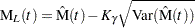
Default approximate two-sided $\text{[math]}$ pointwise confidence limits for $\text{[math]}$ are computed as

$\text{[math]}$

where $\text{[math]}$ represents the $\text{[math]}$ percentile of the standard normal distribution.

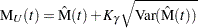
If you specify the LOGINTERVALS option in the MCFPLOT statement, alternative confidence intervals based on the asymptotic normality of $\text{[math]}$ , rather than of $\text{[math]}$ , are computed. Let

$\text{[math]}$

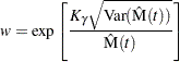Then the limits are computed as

$\text{[math]}$

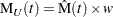These alternative limits are always positive, and can provide better coverage than the default limits when the MCF is known to be positive, such as for counts or for positive costs. They are not appropriate for MCF differences, and are not computed in this case.

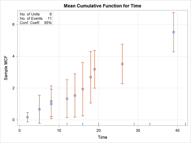
The following SAS statements create the tabular output shown in Figure 14.56 and the plot shown in Figure 14.57:

data Art;               
   input Sysid $ Time Cost; 
   datalines;                  
sys1 19 2               
sys1 39 2               
sys1 42 -1              
sys2 8  2               
sys2 14 1               
sys2 26 1               
sys2 33 -1              
sys3 18 3               
sys3 29 -1              
sys4 16 2               
sys4 2  1               
sys4 20  -1             
sys4 8  1               
sys5 16 -1              
sys6 5 3                
sys6 12 1               
sys6 12 -1              
;

proc reliability data=Art;
   unitid Sysid;
   mcfplot Time*Cost(-1) ;
run;

The first table in Figure 14.56 displays the input data set, the number of observations used in the analysis, the number of systems (units), and the number of repair events. The second table displays the system age, MCF estimate, standard error, approximate confidence limits, and system ID for each event.

Figure 14.56 PROC RELIABILITY Output for the Artificial Data

The RELIABILITY Procedure

Recurrence Data Summary
Input Data Set	WORK.ART
Observations Used	17
Number of Units	6
Number of Events	11

Recurrence Data Analysis
Age	Sample MCF	Standard Error	95% Confidence Limits		Unit ID
Age	Sample MCF	Standard Error	Lower	Upper	Unit ID
2.00	0.167	0.152	-0.132	0.465	sys4
5.00	0.667	0.451	-0.218	1.551	sys6
8.00	1.000	0.471	0.076	1.924	sys2
8.00	1.167	0.495	0.196	2.138	sys4
12.00	1.333	0.609	0.141	2.526	sys6
12.00	.	.	.	.	sys6
14.00	1.533	0.695	0.172	2.895	sys2
16.00	1.933	0.859	0.249	3.618	sys4
16.00	.	.	.	.	sys5
18.00	2.683	0.828	1.061	4.306	sys3
19.00	3.183	0.607	1.993	4.373	sys1
20.00	.	.	.	.	sys4
26.00	3.517	0.634	2.274	4.759	sys2
29.00	.	.	.	.	sys3
33.00	.	.	.	.	sys2
39.00	5.517	0.634	4.274	6.759	sys1
42.00	.	.	.	.	sys1

Figure 14.57 MCF Plot for the Artificial Data

Estimates of the difference between two MCFs $\text{[math]}$ and the variance of the estimator are computed as in Doganaksoy and Nelson (1998). Confidence limits for the MCF difference function are computed in the same way as for the MCF, by using the variance of the MCF difference function estimator.

Recurrent Events Data with Ages Grouped into Intervals

Recurrence data are sometimes grouped into time intervals for convenience, or to reduce the number of data records to be stored and analyzed. Interval recurrence data consist of the number of recurrences and the number of censored units in each time interval.

You can use PROC RELIABILITY to compute and plot MCFs and MCF differences for interval data. Formulas for the MCF estimator $\text{[math]}$ and the variance of the estimator Var $\text{[math]}$ for interval data, as well as examples and interpretations, are given in Nelson (2002, chapter 5). These calculations apply only to the number of recurrences, and not to cost.

Let $\text{[math]}$ be the total number of units, $\text{[math]}$ the number of recurrences in interval $\text{[math]}$ , $\text{[math]}$ , and $\text{[math]}$ the number of units censored into interval $\text{[math]}$ . Then $\text{[math]}$ and the number entering interval 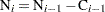$\text{[math]}$ is $\text{[math]}$ with $\text{[math]}$ . The MCF estimate for interval $\text{[math]}$ is $\text{[math]}$ ,

$\text{[math]}$

The denominator $\text{[math]}$ approximates the number at risk in interval $\text{[math]}$ , and treats the censored units as if they were censored halfway through the interval. Since no censored units are likely to have ages lasting through the entire last interval, the MCF estimate for the last interval is likely to be biased. A footnote is printed in the tabular output as a reminder of this bias for the last interval.

See the section Analysis of Interval Age Recurrence Data for an example of interval recurrence data analysis.

Parametric Models for Recurrent Events Data

The parametric models used for recurrent events data in PROC RELIABILITY are called Poisson process models. Some important features of these models are summarized below. See, for example, Rigdon and Basu (2000) and Meeker and Escobar (1998) for a full mathematical description of these models. See Cook and Lawless (2007) for a general discussion of maximum likelihood estimation in Poisson processes. Abernethy (2006) and U.S. Army (2000) provide examples of the application of Poisson process models to system reliability.

Let $\text{[math]}$ be the number of events up to time $\text{[math]}$ , and let $\text{[math]}$ be the number of events in the interval $\text{[math]}$ . Then, for a Poisson process,

$\text{[math]}$ .
$\text{[math]}$ and $\text{[math]}$ are statistically independent if $\text{[math]}$ .
$\text{[math]}$ is a Poisson random variable with mean $\text{[math]}$ where $\text{[math]}$ is the mean number of failures up to time $\text{[math]}$ . $\text{[math]}$ .

Poisson processes are characterized by their cumulative mean function $\text{[math]}$ , or equivalently by their intensity, rate, or rate of occurrence of failure (ROCOF) function $\text{[math]}$ , so that

$\text{[math]}$

Poisson processes are parameterized through their mean and rate functions. The RELIABILITY procedure provides the Poisson process models shown in Table 14.66.

Table 14.66 Models and Parameters for Recurrent Events Data
Model	Intensity Function	Mean Function
Crow-AMSAA	$\text{[math]}$	$\text{[math]}$
Homogeneous	$\text{[math]}$	$\text{[math]}$
Log-linear	$\text{[math]}$	$\text{[math]}$
Power	$\text{[math]}$	$\text{[math]}$
Proportional intensity	$\text{[math]}$	$\text{[math]}$

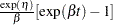
For a homogeneous Poisson process, the intensity function is a constant; that is, the rate of failures does not change with time. For the other models, the rate function can change with time, so that a rate of failures that increases or decreases with time can be modeled. These models are called nonhomogeneous Poisson processes.

In the RELIABILITY procedure, you specify a Poisson model with a DISTRIBUTION statement and a MODEL statement. You must also specify additional statements, depending on whether failure times are observed exactly, or observed to occur in time intervals. These statements are explained in the sections Recurrent Events Data with Exact Event Ages, Recurrent Events Data with Interval Event Ages, and MODEL Statement. The DISTRIBUTION statement specifications for the models described in Table 14.66 are summarized in Table 14.67.

Table 14.67 DISTRIBUTION Statement Specification for Recurrent Events Data Models
Model	DISTRIBUTION Statement Value
Crow-AMSAA	NHPP(CA)
Homogeneous	HPP
Log-linear	NHPP(LOG)
Power	NHPP(POW)
Proportional intensity	NHPP(PROP)

For each of the models, you can specify a regression model for the parameter $\text{[math]}$ in Table 14.66 for the $\text{[math]}$ th observation as

$\text{[math]}$

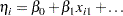where $\text{[math]}$ are regression coefficients specified as described in the section MODEL Statement. The parameter $\text{[math]}$ is labeled Intercept in the printed output, and the parameter $\text{[math]}$ in Table 14.66 is labeled Shape. If no regression coefficients are specified, Intercept represents the parameter $\text{[math]}$ in Table 14.66.

Model parameters are estimated by maximizing the log-likelihood function, which is equivalent to maximizing the likelihood function. The sections Recurrent Events Data with Exact Event Ages and Recurrent Events Data with Interval Event Ages contain descriptions of the form of the log likelihoods for the different models. An estimate of the covariance matrix of the maximum likelihood estimators (MLEs) of the parameters $\text{[math]}$ is given by the inverse of the negative of the matrix of second derivatives of the log likelihood, evaluated at the final parameter estimates:

$\text{[math]}$

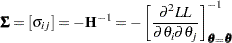The negative of the matrix of second derivatives is called the observed Fisher information matrix. The diagonal term $\text{[math]}$ is an estimate of the variance of $\text{[math]}$ . Estimates of standard errors of the MLEs are provided by

$\text{[math]}$

An estimator of the correlation matrix is

$\text{[math]}$

Wald-type confidence intervals are computed for the model parameters as described in Table 14.68. Wald intervals use asymptotic normality of maximum likelihood estimates to compute approximate confidence intervals. If a parameter must be greater than zero, then an approximation based on the asymptotic normality of the logarithm of the parameter estimate is often more accurate, and the lower endpoint is strictly positive. The intercept term $\text{[math]}$ in an intercept-only power NHPP model with no other regression parameters represents $\text{[math]}$ in Table 14.66, and is a model parameter that must be strictly positive. Also, the shape parameter for the power and proportional intensity models, represented by $\text{[math]}$ in Table 14.66, must be strictly positive. In these cases, formula 7.11 of Meeker and Escobar (1998, p. 163) is used in Table 14.68 to compute confidence limits.

Table 14.68 shows the method of computation of approximate two-sided $\text{[math]}$ confidence limits for model parameters. The default value of confidence is $\text{[math]}$ . Other values of confidence are specified using the CONFIDENCE= option. In Table 14.68, $\text{[math]}$ represents the $\text{[math]}$ percentile of the standard normal distribution, and $\text{[math]}$ .

Table 14.68 NHPP Model Parameter Confidence Limit Computation
		Parameters
Model		Intercept	Regression	Shape
			Parameters
Crow-AMSAA
Intercept-only model
	$\text{[math]}$	$\text{[math]}$		$\text{[math]}$
	$\text{[math]}$	$\text{[math]}$		$\text{[math]}$
Regression model
	$\text{[math]}$	$\text{[math]}$	$\text{[math]}$	$\text{[math]}$
	$\text{[math]}$	$\text{[math]}$	$\text{[math]}$	$\text{[math]}$
Homogeneous
	$\text{[math]}$	$\text{[math]}$	$\text{[math]}$
	$\text{[math]}$	$\text{[math]}$	$\text{[math]}$
Log-linear
	$\text{[math]}$	$\text{[math]}$	$\text{[math]}$	$\text{[math]}$
	$\text{[math]}$	$\text{[math]}$	$\text{[math]}$	$\text{[math]}$
Power
Intercept-only model
	$\text{[math]}$	$\text{[math]}$		$\text{[math]}$
	$\text{[math]}$	$\text{[math]}$		$\text{[math]}$
Regression model
	$\text{[math]}$	$\text{[math]}$	$\text{[math]}$	$\text{[math]}$
	$\text{[math]}$	$\text{[math]}$	$\text{[math]}$	$\text{[math]}$
Proportional intensity
	$\text{[math]}$	$\text{[math]}$	$\text{[math]}$	$\text{[math]}$
	$\text{[math]}$	$\text{[math]}$	$\text{[math]}$	$\text{[math]}$

You can request that profile likelihood confidence intervals for model parameters be computed instead of Wald intervals with the LRCL option in the MODEL statement.

For the nonhomogeneous models in Table 14.66, you can request a test for a homogeneous Poisson process by specifying the HPPTEST option in the MODEL statement. In this case the test is a likelihood ratio test for $\text{[math]}$ for the power, Crow-AMSAA, and proportional intensity models, and $\text{[math]}$ for the log-linear model.

INEST Data Set for Recurrent Events Models

You can specify a SAS data set to set lower bounds, upper bounds, equality constraints, or initial values for estimating the intercept and shape parameters of the models in Table 14.66 by using the INEST= option in the MODEL statement. The data set must contain a variable named _TYPE_ that specifies the action that you want to take in the iterative estimation process, and some combination of variables named _INTERCEPT_ and _SHAPE_ that represent the distribution parameters. If BY processing is used, the INEST= data set should also include the BY variables, and there must be at least one observation for each BY group.

The possible values of _TYPE_ and corresponding actions are summarized in Table 14.69.

Table 14.69 _TYPE_ Variable Values
Value of _TYPE_	Action
LB	Lower bound
UB	Upper bound
EQ	Equality
PARMS	Initial value

For example, you can use the INEST data set In created by the following SAS statements to specify an equality constraint for the shape parameter. The data set In specifies that the shape parameter be constrained to be 1.5. Since the variable _Intercept_ is set to missing, no action is taken for it, and this variable could be omitted from the data set.

data In ;
   input _Type_$ 1-5  _Intercept_  _Shape_;
   datalines;
eq    . 1.5  
;

Recurrent Events Data with Exact Event Ages

Let there be $\text{[math]}$ independent systems observed, and let $\text{[math]}$ be the times of observed events for system $\text{[math]}$ . Let the last time of observation of system $\text{[math]}$ be $\text{[math]}$ , with $\text{[math]}$ .

If there are no regression parameters in the model, or there are regression parameters and they are constant for each system, then the log-likelihood function is

$\text{[math]}$

If there are regression parameters that can change over time for individual systems, the RELIABILITY procedure uses the convention that a covariate value specified at a given event time takes effect immediately after the event time; that is, the value of a covariate used at an event time is the value specified at the previous event time. The value used at the first event time is the value specified at that event time. You can establish a different value for the first event time by specifying a zero cost event previous to the first actual event. The zero cost event is not used in the analysis, but it is used to establish a covariate value for the next event time. The covariate value used at the end time $\text{[math]}$ is the value established at the last event time.

With these conventions, the log likelihood is

$\text{[math]}$

with $\text{[math]}$ for each $\text{[math]}$ . Note that this log likelihood reduces to the previous log likelihood if covariate values do not change over time for each system.

In order to specify a parametric model for recurrence data with exact event times, you specify the event times, end of observation times, and regression model, if any, with a MODEL statement, as described in the section MODEL Statement. In addition, you specify a variable that uniquely identifies each system with a UNITID statement. See the section Parametric Model for Recurrent Events Data for an example of fitting a parametric recurrent events model to data with exact recurrence times.

Recurrent Events Data with Interval Event Ages

If $\text{[math]}$ independent and statistically identical systems are observed in the time interval $\text{[math]}$ , then the number $\text{[math]}$ of events that occur in the interval is a Poisson random variable with mean $\text{[math]}$ , where $\text{[math]}$ is the cumulative mean function for an individual system.

Let $\text{[math]}$ be nonoverlapping time intervals for which $\text{[math]}$ events are observed among the $\text{[math]}$ systems observed in time interval $\text{[math]}$ . The parameters in the mean function $\text{[math]}$ are estimated by maximizing the log likelihood

$\text{[math]}$

The time intervals do not have to be of the same length, and they do not have to be adjacent, although the preceding formula shows them as adjacent.

If you have data from groups of systems to which you are fitting a regression model (for example, to model the effects of different manufacturing lines or different vendors), the time intervals in the different groups do not have to coincide. The only requirement is that the data in the different groups be independent; for example, you cannot have data from the same systems in two different groups.

In order to specify a parametric model for interval recurrence data, you specify the time intervals and regression model, if any, with a MODEL statement, as described in the section MODEL Statement. In addition, you specify a variable that contains the number $\text{[math]}$ of systems under observation in time interval $\text{[math]}$ with an NENTER statement, and the number of events $\text{[math]}$ observed with a FREQ statement. See the section Parametric Model for Interval Recurrent Events Data for an example of fitting a parametric recurrent events model to data with interval recurrence times.