PPPLOT Statement: CAPABILITY Procedure

specifies the shape parameter for P-P plots requested with the BETA, GAMMA, PARETO, and POWER options. For examples, see the entries for the distribution options.

creates a beta P-P plot. To create the plot, the nonmissing observations are ordered from smallest to largest:

The -coordinate of the th point is the empirical cdf value . The -coordinate is the theoretical beta cdf value

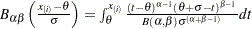
where is the normalized incomplete beta function, 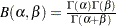, and

lower threshold parameter
scale parameter
first shape parameter
second shape parameter

You can specify , , , and with the ALPHA=, BETA=, SIGMA=, and THETA= beta-options, as illustrated in the following example:

proc capability data=measures;
   ppplot width / beta(theta=1 sigma=2 alpha=3 beta=4);
run;

If you do not specify values for these parameters, then by default, , , and maximum likelihood estimates are calculated for and .

IMPORTANT: If the default unit interval (0,1) does not adequately describe the range of your data, then you should specify THETA= and SIGMA= so that your data fall in the interval .

If the data are beta distributed with parameters , , , and , then the points on the plot for ALPHA=, BETA=, SIGMA=, and THETA= tend to fall on or near the diagonal line , which is displayed by default. Agreement between the diagonal line and the point pattern is evidence that the specified beta distribution is a good fit. You can specify the SCALE= option as an alias for the SIGMA= option and the THRESHOLD= option as an alias for the THETA= option.

specifies the shape parameter for P-P plots requested with the BETA distribution option. See the preceding entry for the BETA distribution option for an example.

specifies the shape parameter for P-P plots requested with the WEIBULL option. See the entry for the WEIBULL option for examples.

creates an exponential P-P plot. To create the plot, the nonmissing observations are ordered from smallest to largest:

The -coordinate of the th point is the empirical cdf value . The -coordinate is the theoretical exponential cdf value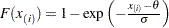

where

threshold parameter
scale parameter

You can specify and with the SIGMA= and THETA= exponential-options, as illustrated in the following example:

proc capability data=measures;
   ppplot width / exponential(theta=1 sigma=2);
run;

If you do not specify values for these parameters, then by default, and a maximum likelihood estimate is calculated for .

IMPORTANT: Your data must be greater than or equal to the lower threshold . If the default is not an adequate lower bound for your data, specify with the THETA= option.

If the data are exponentially distributed with parameters and , the points on the plot for SIGMA= and THETA= tend to fall on or near the diagonal line , which is displayed by default. Agreement between the diagonal line and the point pattern is evidence that the specified exponential distribution is a good fit. You can specify the SCALE= option as an alias for the SIGMA= option and the THRESHOLD= option as an alias for the THETA= option.

creates a gamma P-P plot. To create the plot, the nonmissing observations are ordered from smallest to largest:

The -coordinate of the th point is the empirical cdf value . The -coordinate is the theoretical gamma cdf value

where is the normalized incomplete gamma function, and

threshold parameter
scale parameter
shape parameter

You can specify , , and with the ALPHA=, SIGMA=, and THETA= gamma-options, as illustrated in the following example:

proc capability data=measures;
   ppplot width / gamma(alpha=1 sigma=2 theta=3);
run;

If you do not specify values for these parameters, then by default, and maximum likelihood estimates are calculated for and .

IMPORTANT: Your data must be greater than or equal to the lower threshold . If the default is not an adequate lower bound for your data, specify with the THETA= option.

If the data are gamma distributed with parameters , , and , the points on the plot for ALPHA=, SIGMA=, and THETA= tend to fall on or near the diagonal line , which is displayed by default. Agreement between the diagonal line and the point pattern is evidence that the specified gamma distribution is a good fit. You can specify the SHAPE= option as an alias for the ALPHA= option, the SCALE= option as an alias for the SIGMA= option, and the THRESHOLD= option as an alias for the THETA= option.

creates a Gumbel P-P plot. To create the plot, the nonmissing observations are ordered from smallest to largest:

The -coordinate of the th point is the empirical cdf value . The -coordinate is the theoretical Gumbel cdf value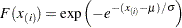

where

location parameter
scale parameter

You can specify and with the MU= and SIGMA= Gumbel-options. By default, maximum likelihood estimates are computed for and .

If the data are Gumbel distributed with parameters and , the points on the plot for MU= and SIGMA= tend to fall on or near the diagonal line , which is displayed by default. Agreement between the diagonal line and the point pattern is evidence that the specified Gumbel distribution is a good fit.

creates an inverse Gaussian P-P plot. To create the plot, the nonmissing observations are ordered from smallest to largest:

The -coordinate of the th point is the empirical cdf value . The -coordinate is the theoretical inverse Gaussian cdf value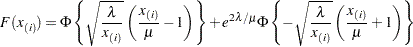

where is the standard normal cumulative distribution function, and

mean parameter
shape parameter

You can specify known values for and with the MU= and LAMBDA= iGauss-options. By default, the sample mean is calculated for and a maximum likelihood estimate is computed for and .

If the data are inverse Gaussian distributed with parameters and , the points on the plot for MU= and LAMBDA= tend to fall on or near the diagonal line , which is displayed by default. Agreement between the diagonal line and the point pattern is evidence that the specified inverse Gaussian distribution is a good fit.

specifies the shape parameter () for P-P plots requested with the IGAUSS option. Enclose the LAMBDA= option in parentheses after the IGAUSS distribution keyword. If you do not specify a value for , the procedure calculates a maximum likelihood estimate.

creates a lognormal P-P plot. To create the plot, the nonmissing observations are ordered from smallest to largest:

The -coordinate of the th point is the empirical cdf value . The -coordinate is the theoretical lognormal cdf value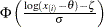

where is the cumulative standard normal distribution function, and

threshold parameter
scale parameter
shape parameter

You can specify , , and with the THETA=, ZETA=, and SIGMA= lognormal-options, as illustrated in the following example:

proc capability data=measures;
   ppplot width / lognormal(theta=1 zeta=2);
run;

If you do not specify values for these parameters, then by default, and maximum likelihood estimates are calculated for and .

IMPORTANT: Your data must be greater than the lower threshold . If the default is not an adequate lower bound for your data, specify with the THETA= option.

If the data are lognormally distributed with parameters , , and , the points on the plot for SIGMA=, THETA=, and ZETA= tend to fall on or near the diagonal line , which is displayed by default. Agreement between the diagonal line and the point pattern is evidence that the specified lognormal distribution is a good fit. You can specify the SHAPE= option as an alias for the SIGMA= option, the SCALE= option as an alias for the ZETA= option, and the THRESHOLD= option as an alias for the THETA= option.

specifies the parameter for a P-P plot requested with the GUMBEL, IGAUSS, and NORMAL options. For examples, see Figure 5.31, or Figure 5.32 and Figure 5.33. For the normal and inverse Gaussian distributions, the default value of is the sample mean. If you do not specify a value for for the Gumbel distribution, the procedure calculates a maximum likelihood estimate.

suppresses the diagonal reference line.

[Line Printer] suppresses the legend that indicates the number of hidden observations.

creates a normal P-P plot. By default, if you do not specify a distribution option, the procedure displays a normal P-P plot. To create the plot, the nonmissing observations are ordered from smallest to largest:

The -coordinate of the th point is the empirical cdf value . The -coordinate is the theoretical normal cdf value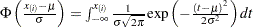

where is the cumulative standard normal distribution function, and

location parameter or mean
scale parameter or standard deviation

You can specify and with the MU= and SIGMA= normal-options, as illustrated in the following example:

proc capability data=measures;
   ppplot width / normal(mu=1 sigma=2);
run;

By default, the sample mean and sample standard deviation are used for and .

If the data are normally distributed with parameters and , the points on the plot for MU= and SIGMA= tend to fall on or near the diagonal line , which is displayed by default. Agreement between the diagonal line and the point pattern is evidence that the specified normal distribution is a good fit. For an example, see Figure 5.31.

creates a generalized Pareto P-P plot. To create the plot, the nonmissing observations are ordered from smallest to largest:

The -coordinate of the th point is the empirical cdf value . The -coordinate is the theoretical generalized Pareto cdf value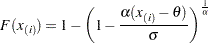

where

threshold parameter
scale parameter
shape parameter

The parameter for the generalized Pareto distribution must be less than the minimum data value. You can specify with the THETA= Pareto-option. The default value for is 0. In addition, the generalized Pareto distribution has a shape parameter and a scale parameter . You can specify these parameters with the ALPHA= and SIGMA= Pareto-options. By default, maximum likelihood estimates are computed for and .

If the data are generalized Pareto distributed with parameters , , and , the points on the plot for THETA=, SIGMA=, and ALPHA= tend to fall on or near the diagonal line , which is displayed by default. Agreement between the diagonal line and the point pattern is evidence that the specified generalized Pareto distribution is a good fit.

creates a power function P-P plot. To create the plot, the nonmissing observations are ordered from smallest to largest:

The -coordinate of the th point is the empirical cdf value . The -coordinate is the theoretical power function cdf value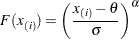

where

lower threshold parameter (lower endpoint)
scale parameter
shape parameter

The power function distribution is bounded below by the parameter and above by the value . You can specify and by using the THETA= and SIGMA= power-options. The default values for and are 0 and 1, respectively.

You can specify a value for the shape parameter, , with the ALPHA= power-option. If you do not specify a value for , the procedure calculates a maximum likelihood estimate.

The power function distribution is a special case of the beta distribution with its second shape parameter, .

If the data are power function distributed with parameters , , and , the points on the plot for THETA=, SIGMA=, and ALPHA= tend to fall on or near the diagonal line , which is displayed by default. Agreement between the diagonal line and the point pattern is evidence that the specified power function distribution is a good fit.

[Line Printer] specifies the character used to plot the points in a line printer plot. The default is the plus sign ().

creates a Rayleigh P-P plot. To create the plot, the nonmissing observations are ordered from smallest to largest:

The -coordinate of the th point is the empirical cdf value . The -coordinate is the theoretical Rayleigh cdf value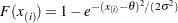

where

threshold parameter
scale parameter

The parameter for the Rayleigh distribution must be less than the minimum data value. You can specify with the THETA= Rayleigh-option. The default value for is 0. You can specify with the SIGMA= Rayleigh-option. By default, a maximum likelihood estimate is computed for .

If the data are Rayleigh distributed with parameters and , the points on the plot for THETA= and SIGMA= tend to fall on or near the diagonal line , which is displayed by default. Agreement between the diagonal line and the point pattern is evidence that the specified Rayleigh distribution is a good fit.

specifies the parameter , where . When used with the BETA, EXPONENTIAL, GAMMA, GUMBEL, NORMAL, PARETO, POWER, RAYLEIGH, and WEIBULL options, the SIGMA= option specifies the scale parameter. When used with the LOGNORMAL option, the SIGMA= option specifies the shape parameter. Enclose the SIGMA= option in parentheses after the distribution keyword. For an example of the SIGMA= option used with the NORMAL option, see Figure 5.31.

displays the P-P plot in a square frame. The default is a rectangular frame. See Figure 5.31 for an example.

[Line Printer] specifies the character used for the diagonal reference line in line printer plots. The default character is the first letter of the distribution option keyword.

specifies the lower threshold parameter for plots requested with the BETA, EXPONENTIAL, GAMMA, LOGNORMAL, PARETO, POWER, RAYLEIGH, and WEIBULL options.

creates a Weibull P-P plot. To create the plot, the nonmissing observations are ordered from smallest to largest:

The -coordinate of the th point is the empirical cdf value . The -coordinate is the theoretical Weibull cdf value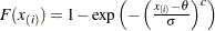

where

threshold parameter
scale parameter
shape parameter

You can specify , , and with the C=, SIGMA=, and THETA= Weibull-options, as illustrated in the following example:

proc capability data=measures;
   ppplot width / weibull(theta=1 sigma=2);
run;

If you do not specify values for these parameters, then by default and maximum likelihood estimates are calculated for and .

IMPORTANT: Your data must be greater than or equal to the lower threshold . If the default is not an adequate lower bound for your data, you should specify with the THETA= option.

If the data are Weibull distributed with parameters , , and , the points on the plot for C=, SIGMA=, and THETA= tend to fall on or near the diagonal line , which is displayed by default. Agreement between the diagonal line and the point pattern is evidence that the specified Weibull distribution is a good fit. You can specify the SHAPE= option as an alias for the C= option, the SCALE= option as an alias for the SIGMA= option, and the THRESHOLD= option as an alias for the THETA= option.

specifies a value for the scale parameter for lognormal P-P plots requested with the LOGNORMAL option.