PPPLOT Statement: CAPABILITY Procedure

Creating a Normal Probability-Probability Plot

[See CAPPP1 in the SAS/QC Sample Library]The distances between two holes cut into 50 steel sheets are measured and saved as values of the variable Distance in the following data set: ¹

data Sheets;
   input Distance @@;
   label Distance='Hole Distance in cm';
   datalines;
 9.80 10.20 10.27  9.70  9.76
10.11 10.24 10.20 10.24  9.63
 9.99  9.78 10.10 10.21 10.00
 9.96  9.79 10.08  9.79 10.06
10.10  9.95  9.84 10.11  9.93
10.56 10.47  9.42 10.44 10.16
10.11 10.36  9.94  9.77  9.36
 9.89  9.62 10.05  9.72  9.82
 9.99 10.16 10.58 10.70  9.54
10.31 10.07 10.33  9.98 10.15
;

The cutting process is in statistical control. As a preliminary step in a capability analysis of the process, it is decided to check whether the distances are normally distributed. The following statements create a P-P plot, shown in Figure 5.31, which is based on the normal distribution with mean and standard deviation :

ods graphics off;
symbol v=plus;
title 'Normal Probability-Probability Plot for Hole Distance';
proc capability data=Sheets noprint;
   ppplot Distance / normal(mu=10 sigma=0.3)
                     square;
run;

The NORMAL option in the PPPLOT statement requests a P-P plot based on the normal cumulative distribution function, and the MU= and SIGMA= normal-options specify and . Note that a P-P plot is always based on a completely specified distribution, in other words, a distribution with specific parameters. In this example, if you did not specify the MU= and SIGMA= normal-options, the sample mean and sample standard deviation would be used for and .

Figure 5.31 Normal P-P Plot with Diagonal Reference Line

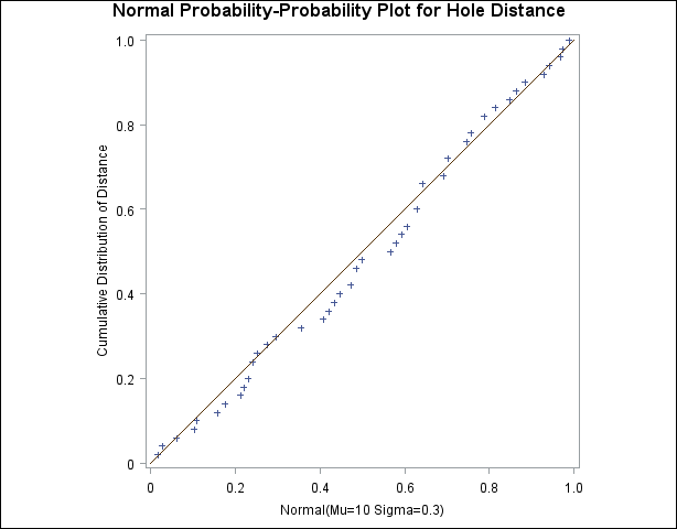
The linearity of the pattern in Figure 5.31 is evidence that the measurements are normally distributed with mean 10 and standard deviation 0.3. The SQUARE option displays the plot in a square format.