| The RELIABILITY Procedure |
| Parameter Estimation and Confidence Intervals |
Maximum Likelihood Estimation
Maximum likelihood estimation of the parameters of a statistical model involves maximizing the likelihood or, equivalently, the log likelihood with respect to the parameters. The parameter values at which the maximum occurs are the maximum likelihood estimates of the model parameters. The likelihood is a function of the parameters and of the data.
Let  be the observations in a random sample, including the failures and censoring times (if the data are censored). Let
  be the probability density of failure time,
  be the reliability function, and
  be the cumulative distribution function, where
  is the vector of parameters to be estimated,
  . The probability density, reliability function, and CDF are determined by the specific distribution selected as a model for the data. The log likelihood is defined as
 |
 |
 |
|||
 |
|
 |
where
 is the sum over failed units
  is the sum over right-censored units
  is the sum over left-censored units
  is the sum over interval-censored units
and  is the interval in which the
  th unit is interval censored. Only the sums appropriate to the type of censoring in the data are included when the preceding equation is used.
The RELIABILITY procedure maximizes the log likelihood with respect to the parameters by using a Newton-Raphson algorithm. The Newton-Raphson algorithm is a recursive method for computing the maximum of a function. On the rth iteration, the algorithm updates the parameter vector  with
with
 |
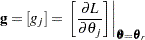
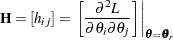
where  is the Hessian (second derivative) matrix, and
  is the gradient (first derivative) vector of the log-likelihood function, both evaluated at the current value of the parameter vector. That is,
 |
and
 |
Iteration continues until the parameter estimates converge. The convergence criterion is
 |
|||
 |
|||
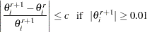 |
for all  where
where  is the convergence criterion. The default value of is
  , and it can be specified with the CONVERGE= option in the MODEL, PROBPLOT, RELATIONPLOT, and ANALYZE statements.
After convergence by the preceding criterion, the quantity
 |
is computed. If  then a warning is printed that the algorithm did not converge.
  is called the relative Hessian convergence criterion. The default value of
  is 0.0001. You can specify other values for with the CONVH= option. The relative Hessian criterion is useful in detecting the occasional case where no progress can be made in increasing the log likelihood, yet the gradient g is not zero.
A location-scale model has a CDF of the form
 |
where  is the location parameter,
  is the scale parameter, and
  is a standardized form
  of the cumulative distribution function. The parameter vector is =( ). It is more convenient computationally to maximize log likelihoods that arise from location-scale models. If you specify a distribution from Table 12.49 that is not a location-scale model, it is transformed to a location-scale model by taking the natural (base
  ) logarithm of the response. If you specify the lognormal base
  distribution, the logarithm (base ) of the response is used. The Weibull, lognormal, and log-logistic distributions in Table 12.49 are not location-scale models. Table 12.50 shows the corresponding location-scale models that result from taking the logarithm of the response.
Maximum likelihood is the default method of estimating the location and scale parameters in the MODEL, PROBPLOT, RELATIONPLOT, and ANALYZE statements. If the Weibull distribution is specified, the logarithms of the responses are used to obtain maximum likelihood estimates (
 ) of the location and scale parameters of the extreme value distribution. The maximum likelihood estimates (
 ,
,  ) of the Weibull scale and shape parameters are computed as
  and
and  .
.
Regression Models
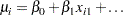
You can specify a regression model by using the MODEL statement. For example, if you want to relate the lifetimes of electronic parts in a test to Arrhenius-transformed operating temperature, then an appropriate model might be
 |
where  , and
, and  is the centigrade temperature at which the th unit is tested. Here,
  [ 1
[ 1  ].
].
There are two types of explanatory variables: continuous variables and classification variables. Continuous variables represent physical quantities, such as temperature or voltage, and they must be numeric. Continuous explanatory variables are sometimes called covariates.
Classification variables identify classification levels and are declared in the CLASS statement. These are also referred to as categorical, dummy, qualitative, discrete, or nominal variables. Classification variables can be either character or numeric. The values of classification variables are called levels. For example, the classification variable Batch could have levels ‘batch1’ and ‘batch2’ to identify items from two production batches. An indicator (0-1) variable is generated for each level of a classification variable and is used as an explanatory variable. See Nelson (1990, p. 277) for an example that uses an indicator variable in the analysis of accelerated life test data. In a model, an explanatory variable that is not declared in a CLASS statement is assumed to be continuous.
By default, all regression models automatically contain an intercept term; that is, the model is of the form
 |
where  does not have an explanatory variable multiplier. The intercept term can be excluded from the model by specifying INTERCEPT
 as a MODEL statement option.
For numerical stability, continuous explanatory variables are centered and scaled internally to the procedure. This transforms the parameters  in the original model to a new set of parameters. The parameter estimates and covariances are transformed back to the original scale before reporting, so that the parameters should be interpreted in terms of the originally specified model. Covariates that are indicator variables—that is, those specified in a CLASS statement—are not centered and scaled.
Initial values of the regression parameters used in the Newton-Raphson method are computed by ordinary least squares. The parameters and the scale parameter are jointly estimated by maximum likelihood, taking a logarithmic transformation of the responses, if necessary, to get a location-scale model.
The generalized gamma distribution is fit using log lifetime as the response variable. The regression parameters , the scale parameter , and the shape parameter  are jointly estimated.
The Weibull distribution shape parameter estimate is computed as , where is the scale parameter from the corresponding extreme value distribution. The Weibull scale parameter  is not computed by the procedure. Instead, the regression parameters and the shape
  are reported.
In a model with one to three continuous explanatory variables  , you can use the RELATION= option in the MODEL statement to specify a transformation that is applied to the variables before model fitting. Table 12.58 shows the available transformations.
Relation |
Transformed variable |
|---|---|
ARRHENIUS (Nelson parameterization) |
|
ARRHENIUS2 (activation energy parameterization) |
|
POWER |
|
LINEAR |
|
LOGISTIC |
|

Nonconstant Scale Parameter
In some situations, it is desirable for the scale parameter to change with the values of explanatory variables. For example, Meeker and Escobar (1998, section 17.5) present an analysis of accelerated life test data where the spread of the data is greater at lower levels of the stress. You can use the LOGSCALE statement to specify the scale parameter as a function of explanatory variables. You must also have a MODEL statement to specify the location parameter. Explanatory variables can be continuous variables, indicator variables specified in the CLASS statement, or any interaction combination. The variables can be the same as specified in the MODEL statement, or they can be different variables. Any transformation specified with the RELATION= MODEL statement option will be applied to the same variable appearing in the LOGSCALE statement. See the section Regression Model with Nonconstant Scale for an example of fitting a model with nonconstant scale parameter.
The form of the model for the scale parameter is
 |
where is the intercept term. The intercept term can be excluded from the model by specifying INTERCEPT as a LOGSCALE statement option.
The parameters  are estimated by maximum likelihood jointly with all the other parameters in the model.
Stable Parameters
The location and scale parameters  are estimated by maximizing the likelihood function by numerical methods, as described previously. An alternative parameterization that is likely to have better numerical properties for heavy censoring is
  , where
  and
and  is the
  th quantile of the standardized distribution. See Meeker and Escobar (1998, p. 90) and Doganaksoy and Schmee (1993) for more details on alternate parameterizations.
By default, RELIABILITY estimates a value of from the data that will improve the numerical properties of the estimation. You can also specify values of from which the value of will be computed with the PSTABLE= option in the ANALYZE, PROBPLOT, RELATIONPLOT, or MODEL statement. Note that a value of  for the Weibull and extreme value and
  for all other distributions will give
  and the parameterization will then be the usual location-scale parameterization.
All estimates and related statistics are reported in terms of the location and scale parameters . If you specify the ITPRINT option in the ANALYZE, PROBPLOT, or RELATIONPLOT statement, a table showing the values of ,  , , and the last evaluation of the gradient and Hessian for these parameters is produced.
Covariance Matrix
An estimate of the covariance matrix of the maximum likelihood estimators (MLEs) of the parameters is given by the inverse of the negative of the matrix of second derivatives of the log likelihood, evaluated at the final parameter estimates:
 |
The negative of the matrix of second derivatives is called the Fisher information matrix. The diagonal term  is an estimate of the variance of
  . Estimates of standard errors of the MLEs are provided by
 |
An estimator of the correlation matrix is
 |
The covariance matrix for the Weibull distribution parameter estimators is computed by a first-order approximation from the covariance matrix of the estimators of the corresponding extreme value parameters as
 |
|
 |
|||
 |
|
 |
|||
 |
|
 |
For the regression model, the variance of the Weibull shape parameter estimator is computed from the variance of the estimator of the extreme value scale parameter as shown previously. The covariance of the regression parameter estimator  and the Weibull shape parameter estimator is computed in terms of the covariance between and as
 |
Confidence Intervals for Distribution Parameters
Table 12.59 shows the method of computation of approximate two-sided  confidence limits for distribution parameters. The default value of confidence is
  . Other values of confidence are specified using the CONFIDENCE= option. In Table 12.59,
  represents the
  percentile of the standard normal distribution, and and are the MLEs of the location and scale parameters for the normal, extreme value, and logistic distributions. For the lognormal, Weibull, and log-logistic distributions, and represent the MLEs of the corresponding location and scale parameters of the location-scale distribution that results when the logarithm of the lifetime is used as the response. For the Weibull distribution, and are the location and scale parameters of the extreme value distribution for the logarithm of the lifetime.
  denotes the standard error of the MLE of
  , computed as the square root of the appropriate diagonal element of the inverse of the Fisher information matrix.
Parameters |
|||
|---|---|---|---|
Distribution |
Location |
Scale |
Shape |
Normal |
|
|
|
|
|
||
Lognormal |
|
|
|
|
|
||
Lognormal |
|
|
|
(base 10) |
|
|
|
Extreme Value |
|
|
|
|
|
||
Weibull |
|
|
|
|
|
||
Exponential |
|
|
|
|
|
||
Logistic |
|
|
|
|
|
||
Log-logistic |
|
|
|
|
|
||
Generalized |
|
|
|
gamma |
|
|
|


Regression Parameters
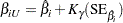
Approximate confidence limits for the regression parameter  are given by
 |
 |
Percentiles
The maximum likelihood estimate of the  percentile
  for the extreme value, normal, and logistic distributions is given by
 |
where  , is the standardized CDF shown in Table 12.60, and
  are the maximum likelihood estimates of the location and scale parameters of the distribution. The maximum likelihood estimate of the percentile
  for the Weibull, lognormal, and log-logistic distributions is given by
 |
where , and is the standardized CDF of the location-scale model corresponding to the logarithm of the response. For the lognormal (base 10) distribution,
 |
Location-Scale |
Location-Scale |
|
|---|---|---|
Distribution |
Distribution |
CDF |
Weibull |
Extreme Value |
|
Lognormal |
Normal |
|
Log-logistic |
Logistic |
|


Confidence Intervals
The variance of the MLE of the  percentile for the normal, extreme value, or logistic distribution is
 |
Two-sided approximate  confidence limits for are
 |
|
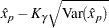 |
|||
 |
|
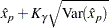 |
where represents the  percentile of the standard normal distribution.
The limits for the lognormal, Weibull, or log-logistic distributions are
 |
|
 |
|||
 |
|
 |
where refers to the percentile of the corresponding location-scale distribution (normal, extreme value, or logistic) for the logarithm of the lifetime. For the lognormal (base 10) distribution,
|
|
 |
|||
|
|
 |
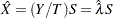
Reliability Function
For the extreme value, normal, and logistic distributions shown in Table 12.60, the maximum likelihood estimate of the reliability function  is given by
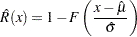 |
The MLE of the CDF is  .
.
Confidence Intervals
Let  . The variance of
  is
is
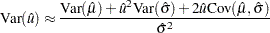 |
Two-sided approximate confidence intervals for  are computed as
 |
 |
where
 |
 |
and represents the percentile of the standard normal distribution.
The corresponding limits for the CDF are
 |
 |
Limits for the Weibull, lognormal, and log-logistic reliability function  are the same as those for the corresponding extreme value, normal, or logistic reliability
  , where
  .
.
You can create a table containing estimates of the reliability function, the CDF, and confidence limits computed as described in this section with the SURVTIME= option in the ANALYZE statement or with the SURVTIME= option in the PROBPLOT statement. You can plot confidence limits for the CDF on probability plots created with the PROBPLOT statement with the PINTERVALS=CDF option in the PROBPLOT statement. PINTERVALS=CDF is the default option for parametric confidence limits on probability plots.
Estimation with the Binomial and Poisson Distributions
In addition to estimating the parameters of the distributions in Table 12.49, you can estimate parameters, compute confidence limits, compute predicted values and prediction limits, and compute chi-square tests for differences in groups for the binomial and Poisson distributions by using the ANALYZE statement. Specify either BINOMIAL or POISSON in the DISTRIBUTION statement to use one of these distributions. The ANALYZE statement options available for the binomial and Poisson distributions are given in Table 12.5. See the section Analysis of Binomial Data for an example of an analysis of binomial data.
Binomial Distribution
If  is the number of successes and
  is the number of trials in a binomial experiment, then the maximum likelihood estimator of the probability in the binomial distribution is computed as
 |
Two-sided confidence limits for are computed as in Johnson, Kotz, and Kemp (1992, p. 130):
 |
with  and
and 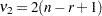 and
and
 |
with  and
and  , where
  is the percentile of the
  distribution with
  degrees of freedom in the numerator and
  degrees of freedom in the denominator.
You can compute a sample size required to estimate within a specified tolerance  with probability
  . Nelson (1982, p. 206) gives the following formula for the approximate sample size:
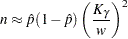 |
where is the percentile of the standard normal distribution. The formula is based on the normal approximation for the distribution of  . Nelson recommends using this formula if
  and
and  . The value of used for computing confidence limits is used in the sample size computation. The default value of confidence is . Other values of confidence are specified using the CONFIDENCE= option. You specify a tolerance of number with the TOLERANCE(number) option.
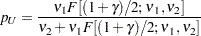
The predicted number of successes  in a future sample of size
  , based on the previous estimate of , is computed as
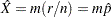 |
Two-sided approximate  prediction limits are computed as in Nelson (1982, p. 208) . The prediction limits are the solutions
  and
and  of
of
 |
 |
where is the  % percentile of the distribution with degrees of freedom in the numerator and degrees of freedom in the denominator. You request predicted values and prediction limits for a future sample of size number with the PREDICT(number) option.
You can test groups of binomial data for equality of their binomial probability by using the ANALYZE statement. You specify the  groups to be compared with a group variable having levels.
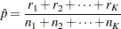
Nelson (1982, p. 450) discusses a chi-square test statistic for comparing binomial proportions for equality. Suppose there are  successes in
  trials for
  . The grouped estimate of the binomial probability is
 |
The chi-square test statistic for testing the hypothesis  against
  for some and
  is
is
 |
The statistic  has an asymptotic chi-square distribution with
  degrees of freedom. The RELIABILITY procedure computes the contribution of each group to , the value of , and the p-value for based on the limiting chi-square distribution with degrees of freedom. If you specify the PREDICT option, predicted values and prediction limits are computed for each group, as well as for the pooled group. The p-value is defined as
  , where
  is the chi-square CDF with degrees of freedom, and is the observed value. A test of the hypothesis of equal binomial probabilities among the groups with significance level
  is
is
 : do not reject the equality hypothesis
  : reject the equality hypothesis
Poisson Distribution
You can use the ANALYZE statement to model data by using the Poisson distribution. The data consist of a count  of occurrences in a "length" of observation
  . Observation is typically an exposure time, but it can have other units, such as distance. The ANALYZE statement enables you to compute the rate of occurrences, confidence limits, and prediction limits.
An estimate of the rate is computed as
 |
Two-sided confidence limits for are computed as in Nelson (1982, p. 201):
 |
 |
where  is the
  percentile of the chi-square distribution with degrees of freedom.
You can compute a length required to estimate within a specified tolerance with probability . Nelson (1982, p. 202) provides the following approximate formula:
 |
where is the percentile of the standard normal distribution. The formula is based on the normal approximation for  and is more accurate for larger values of
  . Nelson recommends using the formula when
  . The value of used for computing confidence limits is also used in the length computation. The default value of confidence is . Other values of confidence are specified using the CONFIDENCE= option. You specify a tolerance of number with the TOLERANCE(number) option.
The predicted future number of occurrences in a length  is
is
 |
Two-sided approximate prediction limits are computed as in Nelson (1982, p. 203). The prediction limits are the solutions and of
 |
 |
where is the percentile of the distribution with degrees of freedom in the numerator and degrees of freedom in the denominator. You request predicted values and prediction limits for a future exposure number with the PREDICT(number) option.
You can compute a chi-square test statistic for comparing Poisson rates for equality. You specify the groups to be compared with a group variable having levels.
See Nelson (1982, p. 444) for more information. Suppose that there are  Poisson counts in lengths for and that the are independent. The grouped estimate of the Poisson rate is
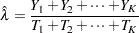 |
The chi-square test statistic for testing the hypothesis  against
  for some and is
 |
The statistic has an asymptotic chi-square distribution with degrees of freedom. The RELIABILITY procedure computes the contribution of each group to , the value of , and the p-value for based on the limiting chi-square distribution with degrees of freedom. If you specify the PREDICT option, predicted values and prediction limits are computed for each group, as well as for the pooled group. The p-value is defined as , where is the chi-square CDF with degrees of freedom and is the observed value. A test of the hypothesis of equal Poisson rates among the groups with significance level is
- : accept the equality hypothesis
- : reject the equality hypothesis
Least Squares Fit to the Probability Plot
Fitting to the probability plot by least squares is an alternative to maximum likelihood estimation of the parameters of a life distribution. Only the failure times are used. A least squares fit is computed using points  , where
  and
and  are the plotting positions as defined in the section Probability Plotting. The are either the lifetimes for the normal, extreme value, or logistic distributions or the log lifetimes for the lognormal, Weibull, or log-logistic distributions. The ANALYZE, PROBPLOT, or RELATIONPLOT statement option FITTYPE=LSXY specifies the
  as the dependent variable (’y-coordinate’) and the
  as the independent variable (’x-coordinate’). You can optionally reverse the quantities used as dependent and independent variables by specifying the FITTYPE=LSYX option.
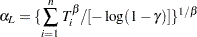
Weibayes Estimation
Weibayes estimation is a method of performing a Weibull analysis when there are few or no failures. The FITTYPE=WEIBAYES option requests this method. The method of Nelson (1985) is used to compute a one-sided confidence interval for the Weibull scale parameter when the Weibull shape parameter is specified. See Abernethy (2006) for more discussion and examples. The Weibull shape parameter is assumed to be known and is specified to the procedure with the SHAPE=number option. Let  be the failure and censoring times, and let
  be the number of failures in the data. If there are no failures
  , a lower confidence limit for the Weibull scale parameter is computed as
 |
The default value of confidence is . Other values of confidence are specified using the CONFIDENCE= option.
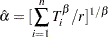
If  , the MLE of is given by
 |
and a lower confidence limit for the Weibull scale parameter is computed as
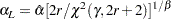 |
where  is the percentile of a chi-square distribution with
  degrees of freedom. The procedure uses the specified value of and the computed value of
  to compute distribution percentiles and the reliability function.
Estimation With Multiple Failure Modes
In many applications, units can experience multiple causes of failure, or failure modes. For example, in the section Weibull Probability Plot for Two Combined Failure Modes, insulation specimens can experience either early failures due to manufacturing defects or degradation failures due to aging. The FMODE statement is used to analyze this type of data. See the section FMODE Statement for the syntax of the FMODE statement. This section describes the analysis of data when units experience multiple failure modes. The assumptions used in the analysis are
a cause, or mode, can be identified for each failure
failure modes follow a series-system model; i.e., a unit fails when a failure due to one of the modes occurs
each failure mode has the specified lifetime distribution with different parameters
failure modes act statistically independently
Suppose there are failure modes, with lifetime distribution functions  .
.
If you wish to estimate the lifetime distribution of a failure mode, say mode , acting alone, specify the KEEP keyword in the FMODE statement. The failures from all other modes are treated as right-censored observations, and the lifetime distribution is estimated by one of the methods described in other sections, such as maximum likelihood. This lifetime distribution is interpreted as the distribution if the specified failure mode is acting alone, with all other modes eliminated. You can also specify more than one mode to KEEP, but the assumption is that all the specified modes have the same distribution.
If you specify the ELIMINATE keyword, failures due to the specified modes are treated as right censored. The resulting distribution estimate is the failure distribution if the specified modes are eliminated.
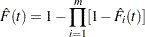
If you specify the COMBINE keyword, the failure distribution when all the modes specified in the FMODE statement modes act is estimated. The failure distribution  , from each individual mode is first estimated by treating all failures from other modes as right censored. The estimated failure distributions are then combined to get an estimate of the lifetime distribution when all modes act,
 |
Pointwise approximate asymptotic normal confidence limits for  can be obtained by the delta method. See Meeker and Escobar (1998, appendix B.2). The delta method variance of
  is, assuming independence of failure modes,
 |
where  ,
,  is
is  for the extreme value, normal, and logistic distributions or
  for the Weibull, lognormal or loglogistic distributions,
  and
and  are location and scale parameter estimates for mode , and
  and
and  are the standard (
 ) survival function and density function for the specified distribution.
Two-sided approximate  pointwise confidence intervals are computed as in Meeker and Escobar (1998, section 3.6) as
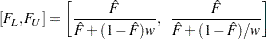 |
where
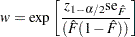 |
where  and
and  is the th quantile of the standard normal distribution.
Copyright © SAS Institute, Inc. All Rights Reserved.