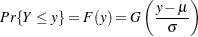
| The RELIABILITY Procedure |
| Probability Plotting |
Probability plots are useful tools for the display and analysis of lifetime data. See Abernethy (2006) for examples that use probability plots in the analysis of reliability data. Probability plots use a special scale so that a cumulative distribution function (CDF) plots as a straight line. Thus, if lifetime data are a sample from a distribution, the CDF estimated from the data plots approximately as a straight line on a probability plot for the distribution.
You can use the RELIABILITY procedure to construct probability plots for data that are complete, right censored, or interval censored (in readout form) for each of the probability distributions in Table 12.49.
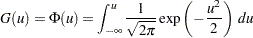
A random variable  belongs to a location-scale family of distributions if its CDF
  is of the form
 |
where  is the location parameter, and
  is the scale parameter. Here,
  is a CDF that cannot depend on any unknown parameters, and is the CDF of if
  and
and  . For example, if is a normal random variable with mean and standard deviation ,
 |
and
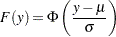 |
Of the distributions in Table 12.49, the normal, extreme value, and logistic distributions are location-scale models. As shown in Table 12.50, if  has a lognormal, Weibull, or log-logistic distribution, then
  has a distribution that is a location-scale model. Probability plots are constructed for lognormal, Weibull, and log-logistic distributions by using instead of in the plots.
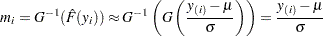
Let 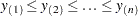 be ordered observations of a random sample with distribution function
  . A probability plot is a plot of the points
  against
  , where
  is an estimate of the CDF
 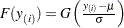 . The points
  are called plotting positions. The axis on which the points
  s are plotted is usually labeled with a probability scale (the scale of ).
If is one of the location-scale distributions, then  is the lifetime; otherwise, the log of the lifetime is used to transform the distribution to a location-scale model.
If the data actually have the stated distribution, then  ,
,
 |
and points  should fall approximately on a straight line.
There are several ways to compute plotting positions from failure data. These are discussed in the next two sections.
Complete and Right-Censored Data
The censoring times must be taken into account when you compute plotting positions for right-censored data. The RELIABILITY procedure provides several methods for computing plotting positions. These are specified with the PPOS= option in the ANALYZE, PROBPLOT, and RELATIONPLOT statements. All of the methods give similar results, as illustrated in the section Expected Ranks, Kaplan-Meier, and Modified Kaplan-Meier Methods, the section Nelson-Aalen, and the section Median Ranks.
Expected Ranks, Kaplan-Meier, and Modified Kaplan-Meier Methods
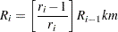
Let be ordered observations of a random sample including failure times and censor times. Order the data in increasing order. Label all the data with reverse ranks  , with
  . For the failure corresponding to reverse rank , compute the reliability, or survivor function estimate
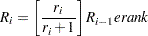 |
with  . The expected rank plotting position is computed as
  . The option PPOS=EXPRANK specifies the expected rank plotting position.
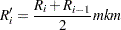
For the Kaplan-Meier method,
 |
The Kaplan-Meier plotting position is then computed as  . The option PPOS=KM specifies the Kaplan-Meier plotting position.
For the modified Kaplan-Meier method, use
 |
where  is computed from the Kaplan-Meier formula with . The plotting position is then computed as
  . The option PPOS=MKM specifies the modified Kaplan-Meier plotting position. If the PPOS option is not specified, the modified Kaplan-Meier plotting position is used as the default method.
For complete samples,  for the expected rank method,
  for the Kaplan-Meier method, and
  for the modified Kaplan-Meier method. If the largest observation is a failure for the Kaplan-Meier estimator, then
  and the point is not plotted. These three methods are shown for the field winding data in Table 12.52 and Table 12.53.
Ordered |
Reverse |
|
|
|
|
|---|---|---|---|---|---|
Observation |
Rank |
||||
31.7 |
16 |
16/17 |
1.0000 |
0.9411 |
0.0588 |
39.2 |
15 |
15/16 |
0.9411 |
0.8824 |
0.1176 |
57.5 |
14 |
14/15 |
0.8824 |
0.8235 |
0.1765 |
65.0+ |
13 |
||||
65.8 |
12 |
12/13 |
0.8235 |
0.7602 |
0.2398 |
70.0 |
11 |
11/12 |
0.7602 |
0.6968 |
0.3032 |
75.0+ |
10 |
||||
75.0+ |
9 |
||||
87.5+ |
8 |
||||
88.3+ |
7 |
||||
94.2+ |
6 |
||||
101.7+ |
5 |
||||
105.8 |
4 |
4/5 |
0.6968 |
0.5575 |
0.4425 |
109.2+ |
3 |
||||
110.0 |
2 |
2/3 |
0.5575 |
0.3716 |
0.6284 |
130.0+ |
1 |
||||
+ Censored Times |
|||||


Ordered |
Reverse |
|
|
|
|
|
|---|---|---|---|---|---|---|
Observation |
Rank |
|||||
31.7 |
16 |
15/16 |
1.0000 |
0.9375 |
0.0625 |
0.0313 |
39.2 |
15 |
14/15 |
0.9375 |
0.8750 |
0.1250 |
0.0938 |
57.5 |
14 |
13/14 |
0.8750 |
0.8125 |
0.1875 |
0.1563 |
65.0+ |
13 |
|||||
65.8 |
12 |
11/12 |
0.8125 |
0.7448 |
0.2552 |
0.2214 |
70.0 |
11 |
10/11 |
0.7448 |
0.6771 |
0.3229 |
0.2891 |
75.0+ |
10 |
|||||
75.0+ |
9 |
|||||
87.5+ |
8 |
|||||
88.3+ |
7 |
|||||
94.2+ |
6 |
|||||
101.7+ |
5 |
|||||
105.8 |
4 |
3/4 |
0.6771 |
0.5078 |
0.4922 |
0.4076 |
109.2+ |
3 |
|||||
110.0 |
2 |
1/2 |
0.5078 |
0.2539 |
0.7461 |
0.6192 |
130.0+ |
1 |
|||||
+ Censored Times |
||||||


Nelson-Aalen
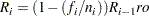
Estimate the cumulative hazard function by
 |
with  . The reliability is
  , and the plotting position, or CDF, is
  . You can show that
  for all ages. The Nelson-Aalen method is shown for the field winding data in Table 12.54.
Ordered |
Reverse |
|
|
|
|
|---|---|---|---|---|---|
Observation |
Rank |
||||
31.7 |
16 |
1/16 |
0.0000 |
0.0625 |
0.0606 |
39.2 |
15 |
1/15 |
0.0625 |
0.1292 |
0.1212 |
57.5 |
14 |
1/14 |
0.1292 |
0.2006 |
0.1818 |
65.0+ |
13 |
||||
65.8 |
12 |
1/12 |
0.2006 |
0.2839 |
0.2472 |
70.0 |
11 |
1/11 |
0.2839 |
0.3748 |
0.3126 |
75.0+ |
10 |
||||
75.0+ |
9 |
||||
87.5+ |
8 |
||||
88.3+ |
7 |
||||
94.2+ |
6 |
||||
101.7+ |
5 |
||||
105.8 |
4 |
1/4 |
0.3748 |
0.6248 |
0.4647 |
109.2+ |
3 |
||||
110.0 |
2 |
1/2 |
0.6248 |
1.1248 |
0.6753 |
130.0+ |
1 |
||||
+ Censored Times |
|||||


Median Ranks
See Abernethy (2006) for a discussion of the methods described in this section. Let be ordered observations of a random sample including failure times and censor times. A failure order number  is assigned to the ith failure:
  , where
  . The increment
  is initially 1 and is modified when a censoring time is encountered in the ordered sample. The new increment is computed as
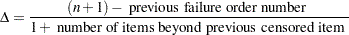 |
The plotting position is computed for the  th failure time as
 |
For complete samples, the failure order number is equal to , the order of the failure in the sample. In this case, the preceding equation for is an approximation to the median plotting position computed as the median of the th-order statistic from the uniform distribution on (0, 1). In the censored case, is not necessarily an integer, but the preceding equation still provides an approximation to the median plotting position. The PPOS=MEDRANK option specifies the median rank plotting position.
For complete data, an alternative method of computing the median rank plotting position for failure is to compute the exact median of the distribution of the th order statistic of a sample of size  from the uniform distribution on (0,1). If the data are right censored, the adjusted rank , as defined in the preceding paragraph, is used in place of in the computation of the median rank. The PPOS=MEDRANK1 option specifies this type of plotting position.
Nelson (1982, p. 148) provides the following example of multiply right-censored failure data for field windings in electrical generators. Table 12.55 shows the data, the intermediate calculations, and the plotting positions calculated by exact ( ) and approximate () median ranks.
Ordered |
Increment |
Failure Order |
||
|---|---|---|---|---|
Observation |
|
Number |
|
|
31.7 |
1.0000 |
1.0000 |
0.04268 |
0.04240 |
39.2 |
1.0000 |
2.0000 |
0.1037 |
0.1027 |
57.5 |
1.0000 |
3.0000 |
0.1646 |
0.1637 |
65.0+ |
1.0769 |
|||
65.8 |
1.0769 |
4.0769 |
0.2303 |
0.2294 |
70.0 |
1.0769 |
5.1538 |
0.2960 |
0.2953 |
75.0+ |
1.1846 |
|||
75.0+ |
1.3162 |
|||
87.5+ |
1.4808 |
|||
88.3+ |
1.6923 |
|||
94.2+ |
1.9744 |
|||
101.7+ |
2.3692 |
|||
105.8 |
2.3692 |
7.5231 |
0.4404 |
0.4402 |
109.2+ |
3.1590 |
|||
110.0 |
3.1590 |
10.6821 |
0.6331 |
0.6335 |
130.0+ |
6.3179 |
|||
+ Censored Times |
||||
Interval-Censored Data
Readout Data
The RELIABILITY procedure can create probability plots for interval-censored data when all units share common interval endpoints. This type of data is called readout data in the RELIABILITY procedure. Estimates of the cumulative distribution function are computed at times corresponding to the interval endpoints. Right censoring can also be accommodated if the censor times correspond to interval endpoints. See the section Weibull Analysis of Interval Data with Common Inspection Schedule for an example of a Weibull plot and analysis for interval data.
Table 12.56 illustrates the computational scheme used to compute the CDF estimates. The data are failure data for microprocessors (Nelson; 1990, p. 147). In Table 12.56,  are the interval upper endpoints, in hours,
  is the number of units failing in interval , and
  is the number of unfailed units at the beginning of interval .
Note that there is right censoring as well as interval censoring in these data. For example, two units fail in the interval (24, 48) hours, and there are 1414 unfailed units at the beginning of the interval, 24 hours. At the beginning of the next interval, (48, 168) hours, there are 573 unfailed units. The number of unfailed units that are removed from the test at 48 hours is  units. These are right-censored units.
The reliability at the end of interval is computed recursively as
 |
with . The plotting position is .
Interval |
Interval |
|
|
|
|
|---|---|---|---|---|---|
|
Endpoint |
|
|
||
1 |
6 |
6/1423 |
0.99578 |
0.99578 |
.00421 |
2 |
12 |
2/1417 |
0.99859 |
0.99438 |
.00562 |
3 |
24 |
0/1415 |
1.00000 |
0.99438 |
.00562 |
4 |
48 |
2/1414 |
0.99859 |
0.99297 |
.00703 |
5 |
168 |
1/573 |
0.99825 |
0.99124 |
.00876 |
6 |
500 |
1/422 |
0.99763 |
0.98889 |
.01111 |
7 |
1000 |
2/272 |
0.99265 |
0.98162 |
.01838 |
8 |
2000 |
1/123 |
0.99187 |
0.97364 |
.02636 |


Arbitrarily Censored Data
The RELIABILITY procedure can create probability plots for data that consists of combinations of exact, left-censored, right-censored, and interval-censored lifetimes. Unlike the method in the previous section, failure intervals need not share common endpoints, although if the intervals share common endpoints, the two methods give the same results. The RELIABILITY procedure uses an iterative algorithm developed by Turnbull (1976) to compute a nonparametric maximum likelihood estimate of the cumulative distribution function for the data. Since the technique is maximum likelihood, standard errors of the cumulative probability estimates are computed from the inverse of the associated Fisher information matrix. A technique developed by Gentleman and Geyer (1994) is used to check for convergence to the maximum likelihood estimate. Also see Meeker and Escobar (1998, chap. 3) for more information.
Although this method applies to more general situations, where the intervals may be overlapping, the example of the previous section will be used to illustrate the method. Table 12.57 contains the microprocessor data of the previous section, arranged in intervals. A missing (.) lower endpoint indicates left censoring, and a missing upper endpoint indicates right censoring. These can be thought of as semi-infinite intervals with lower (upper) endpoint of negative (positive) infinity for left (right) censoring.
Lower |
Upper |
Number |
|---|---|---|
Endpoint |
Endpoint |
Failed |
. |
6 |
6 |
6 |
12 |
2 |
24 |
48 |
2 |
24 |
. |
1 |
48 |
168 |
1 |
48 |
. |
839 |
168 |
500 |
1 |
168 |
. |
150 |
500 |
1000 |
2 |
500 |
. |
149 |
1000 |
2000 |
1 |
1000 |
. |
147 |
2000 |
. |
122 |
The following SAS statements compute the Turnbull estimate and create a lognormal probability plot:
   data micro;
      input t1 t2 f ;
      datalines;
      . 6 6
      6 12 2
      12 24 0
      24 48 2
      24 .  1
      48 168 1
      48 .   839
      168 500 1
      168 .   150
      500 1000 2
      500 .    149
      1000 2000 1
      1000 . 147
      2000 . 122
      ;
   run;
proc reliability data=micro;
   distribution lognormal;
   freq f;
   pplot ( t1 t2 ) / itprintem
                     printprobs
                     maxitem = ( 1000, 25 )
                     nofit
                     npintervals = simul
                     ppout;
run;
The nonparametric maximum likelihood estimate of the CDF can only increase on certain intervals, and must remain constant between the intervals. The Turnbull algorithm first computes the intervals on which the nonparametric maximum likelihood estimate of the CDF can increase. The algorithm then iteratively estimates the probability associated with each interval. The ITPRINTEM option along with the PRINTPROBS option instructs the procedure to print the intervals on which probability increases can occur and the iterative history of the estimates of the interval probabilities. The PPOUT option requests tabular output of the estimated CDF, standard errors, and confidence limits for each cumulative probability.
Figure 12.43 shows every 25th iteration and the last iteration for the Turnbull estimate of the CDF for the microprocessor data. The initial estimate assigns equal probabilities to each interval. You can specify different initial values with the PROBLIST= option. The algorithm converges in 130 iterations for this data. Convergence is determined if the change in the loglikelihood between two successive iterations less than , where the default value is  . You can specify a different value for delta with the TOLLIKE= option. This algorithm is an example of an expectation-maximization (EM) algorithm. EM algorithms are known to converge slowly, but the computations within each iteration for the Turnbull algorithm are moderate. Iterations will be terminated if the algorithm does not converge after a fixed number of iterations. The default maximum number of iterations is 1000. Some data may require more iterations for convergence. You can specify the maximum allowed number of iterations with the MAXITEM= option in the PROBPLOT, ANALYZE, or RPLOT statement.
| Iteration History for the Turnbull Estimate of the CDF | |||||||||
|---|---|---|---|---|---|---|---|---|---|
| Iteration | Loglikelihood | (., 6) | (6, 12) | (24, 48) | (48, 168) | (168, 500) | (500, 1000) | (1000, 2000) | (2000, .) |
| 0 | -1133.4051 | 0.125 | 0.125 | 0.125 | 0.125 | 0.125 | 0.125 | 0.125 | 0.125 |
| 25 | -104.16622 | 0.00421644 | 0.00140548 | 0.00140648 | 0.00173338 | 0.00237846 | 0.00846094 | 0.04565407 | 0.93474475 |
| 50 | -101.15151 | 0.00421644 | 0.00140548 | 0.00140648 | 0.00173293 | 0.00234891 | 0.00727679 | 0.01174486 | 0.96986811 |
| 75 | -101.06641 | 0.00421644 | 0.00140548 | 0.00140648 | 0.00173293 | 0.00234891 | 0.00727127 | 0.00835638 | 0.9732621 |
| 100 | -101.06534 | 0.00421644 | 0.00140548 | 0.00140648 | 0.00173293 | 0.00234891 | 0.00727125 | 0.00801814 | 0.97360037 |
| 125 | -101.06533 | 0.00421644 | 0.00140548 | 0.00140648 | 0.00173293 | 0.00234891 | 0.00727125 | 0.00798438 | 0.97363413 |
| 130 | -101.06533 | 0.00421644 | 0.00140548 | 0.00140648 | 0.00173293 | 0.00234891 | 0.00727125 | 0.007983 | 0.97363551 |
If an interval probability is smaller than a tolerance ( by default) after convergence, the probability is set to zero, the interval probabilities are renormalized so that they add to one, and iterations are restarted. Usually the algorithm converges in just a few more iterations. You can change the default value of the tolerance with the TOLPROB= option. You can specify the NOPOLISH option to avoid setting small probabilities to zero and restarting the algorithm.
If you specify the ITPRINTEM option, the table in Figure 12.44 summarizing the Turnbull estimate of the interval probabilities is printed. The columns labeled ’Reduced Gradient’ and ’Lagrange Multiplier’ are used in checking final convergence to the maximum likelihood estimate. The Lagrange multipliers must all be greater than or equal to zero, or the solution is not maximum likelihood. See Gentleman and Geyer (1994) for more details of the convergence checking.
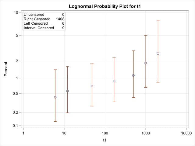
Figure 12.45 shows the final estimate of the CDF, along with standard errors and confidence limits. Figure 12.46 shows the CDF and simultaneous confidence limits plotted on a lognormal probability plot.
| Cumulative Probability Estimates | |||||
|---|---|---|---|---|---|
| Lower Lifetime | Upper Lifetime | Cumulative Probability |
Pointwise 95% Confidence Limits |
Standard Error | |
| Lower | Upper | ||||
| 6 | 6 | 0.0042 | 0.0019 | 0.0094 | 0.0017 |
| 12 | 24 | 0.0056 | 0.0028 | 0.0112 | 0.0020 |
| 48 | 48 | 0.0070 | 0.0038 | 0.0130 | 0.0022 |
| 168 | 168 | 0.0088 | 0.0047 | 0.0164 | 0.0028 |
| 500 | 500 | 0.0111 | 0.0058 | 0.0211 | 0.0037 |
| 1000 | 1000 | 0.0184 | 0.0094 | 0.0357 | 0.0063 |
| 2000 | 2000 | 0.0264 | 0.0124 | 0.0553 | 0.0101 |
Copyright © SAS Institute, Inc. All Rights Reserved.