Example 4.34 Comparing Weibull Quantile Plots

This example compares the use of three-parameter and two-parameter Weibull Q-Q plots for the failure times in months for 48 integrated circuits. The times are assumed to follow a Weibull distribution. The following statements save the failure times as the values of the variable Time in the data set Failures:

data Failures;
   input Time @@;
   label Time = 'Time in Months';
   datalines;
29.42 32.14 30.58 27.50 26.08 29.06 25.10 31.34
29.14 33.96 30.64 27.32 29.86 26.28 29.68 33.76
29.32 30.82 27.26 27.92 30.92 24.64 32.90 35.46
30.28 28.36 25.86 31.36 25.26 36.32 28.58 28.88
26.72 27.42 29.02 27.54 31.60 33.46 26.78 27.82
29.18 27.94 27.66 26.42 31.00 26.64 31.44 32.52
;
run;

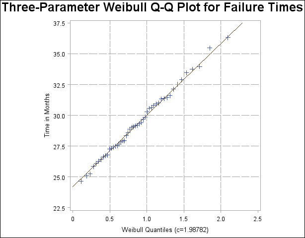
If no assumption is made about the parameters of this distribution, you can use the WEIBULL option to request a three-parameter Weibull plot. As in the previous example, you can visually estimate the shape parameter by requesting plots for different values of and choosing the value of that linearizes the point pattern. Alternatively, you can request a maximum likelihood estimate for , as illustrated in the following statements:

symbol v=plus;
title 'Three-Parameter Weibull Q-Q Plot for Failure Times';
proc univariate data=Failures noprint;
   qqplot Time / weibull(c=est theta=est sigma=est)
                 square
                 href=0.5 1 1.5 2
                 vref=25 27.5 30 32.5 35
                 lhref=4 lvref=4;
run;

Note:When using the WEIBULL option, you must either specify a list of values for the Weibull shape parameter with the C= option or specify C=EST.

Output 4.34.1 displays the plot for the estimated value . The reference line corresponds to the estimated values for the threshold and scale parameters of and , respectively.

Output 4.34.1 Three-Parameter Weibull Q-Q Plot

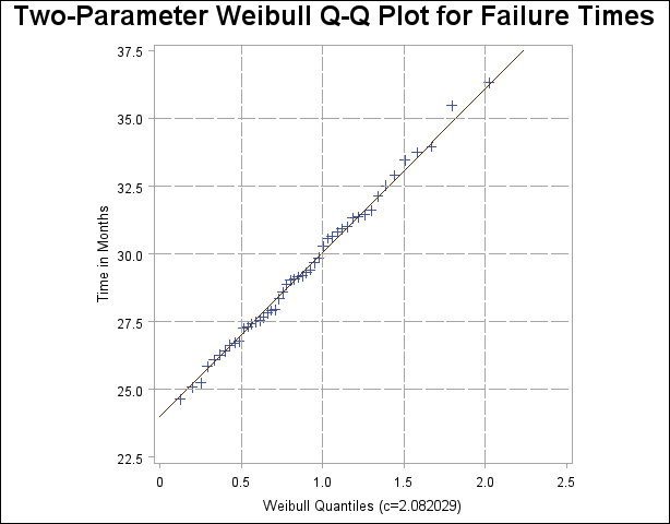
Now, suppose it is known that the circuit lifetime is at least 24 months. The following statements use the known threshold value to produce the two-parameter Weibull Q-Q plot shown in Output 4.31.4:

symbol v=plus;
title 'Two-Parameter Weibull Q-Q Plot for Failure Times';
proc univariate data=Failures noprint;
   qqplot Time / weibull(theta=24 c=est sigma=est)
                 square
                 vref= 25 to 35 by 2.5
                 href= 0.5 to 2.0 by 0.5
                 lhref=4 lvref=4;
run;

The reference line is based on maximum likelihood estimates and .

Output 4.34.2 Two-Parameter Weibull Q-Q Plot for

A sample program for this example, uniex19.sas, is available in the SAS Sample Library for Base SAS software.