Example 4.31 Estimating Three Parameters from Lognormal Quantile Plots

This example, which is a continuation of Example 4.30, demonstrates techniques for estimating the shape, location, and scale parameters, and the theoretical percentiles for a three-parameter lognormal distribution.

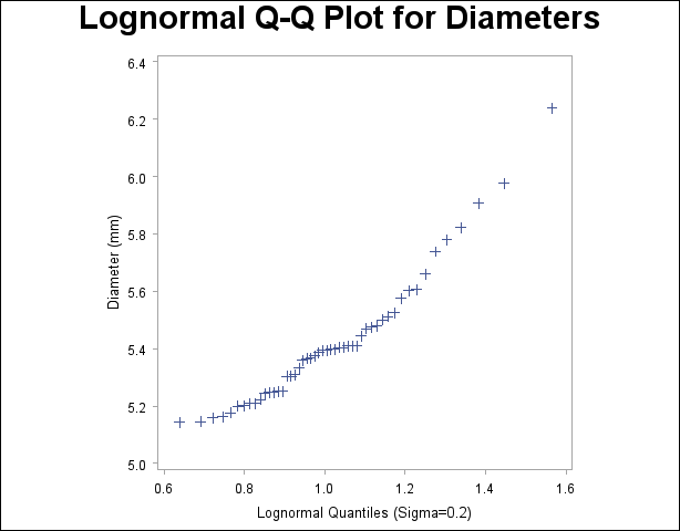
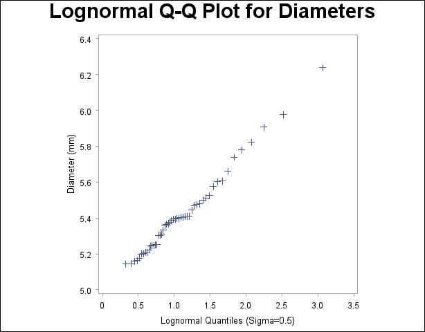
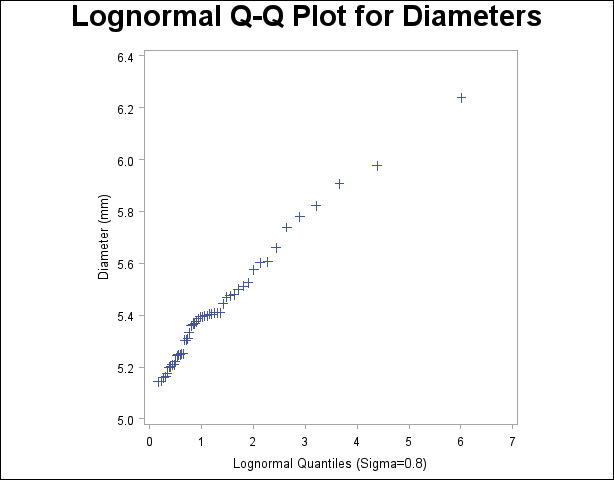
The three-parameter lognormal distribution depends on a threshold parameter , a scale parameter , and a shape parameter . You can estimate from a series of lognormal Q-Q plots which use the SIGMA= secondary option to specify different values of ; the estimate of is the value that linearizes the point pattern. You can then estimate the threshold and scale parameters from the intercept and slope of the point pattern. The following statements create the series of plots in Output 4.31.1, Output 4.31.2, and Output 4.31.3 for values of 0.2, 0.5, and 0.8, respectively:

symbol v=plus;
title 'Lognormal Q-Q Plot for Diameters';
proc univariate data=Measures noprint;
   qqplot Diameter / lognormal(sigma=0.2 0.5 0.8)
                     square;
run;

Note:You must specify a value for the shape parameter for a lognormal Q-Q plot with the SIGMA= option or its alias, the SHAPE= option.

Output 4.31.1 Lognormal Quantile-Quantile Plot ( =0.2)

Output 4.31.2 Lognormal Quantile-Quantile Plot ( =0.5)

Output 4.31.3 Lognormal Quantile-Quantile Plot ( =0.8)

The plot in Output 4.31.2 displays the most linear point pattern, indicating that the lognormal distribution with provides a reasonable fit for the data distribution.

Data with this particular lognormal distribution have the following density function:

The points in the plot fall on or near the line with intercept and slope . Based on Output 4.31.2, and , giving .

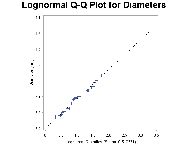
You can also request a reference line by using the SIGMA=, THETA=, and ZETA= options together. The following statements produce the lognormal Q-Q plot in Output 4.31.4:

symbol v=plus;
title 'Lognormal Q-Q Plot for Diameters';
proc univariate data=Measures noprint;
   qqplot Diameter / lognormal(theta=5 zeta=est sigma=est 
                               color=black l=2)
                     square;
run;

Output 4.31.1 through Output 4.31.3 show that the threshold parameter is not equal to zero. Specifying THETA=5 overrides the default value of zero. The SIGMA=EST and ZETA=EST secondary options request estimates for and that use the sample mean and standard deviation.

Output 4.31.4 Lognormal Quantile-Quantile Plot ( =est, =est, =5)

From the plot in Output 4.31.2, can be estimated as 0.51, which is consistent with the estimate of 0.5 derived from the plot in Output 4.31.2. Example 4.32 illustrates how to estimate percentiles by using lognormal Q-Q plots.

A sample program for this example, uniex18.sas, is available in the SAS Sample Library for Base SAS software.