Example 4.32 Estimating Percentiles from Lognormal Quantile Plots

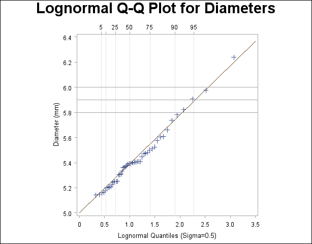
This example, which is a continuation of Example 4.31, shows how to use a Q-Q plot to estimate percentiles such as the 95th percentile of the lognormal distribution. A probability plot can also be used for this purpose, as illustrated in Example 4.26.

The point pattern in Output 4.31.4 has a slope of approximately 0.39 and an intercept of 5. The following statements reproduce this plot, adding a lognormal reference line with this slope and intercept:

symbol v=plus;
title 'Lognormal Q-Q Plot for Diameters';
proc univariate data=Measures noprint;
   qqplot Diameter / lognormal(sigma=0.5 theta=5 slope=0.39)
                     pctlaxis(grid)
                     vref  = 5.8 5.9 6.0
                     square;
run;

The result is shown in Output 4.32.1:

Output 4.32.1 Lognormal Q-Q Plot Identifying Percentiles

The PCTLAXIS option labels the major percentiles, and the GRID option draws percentile axis reference lines. The 95th percentile is 5.9, because the intersection of the distribution reference line and the 95th reference line occurs at this value on the vertical axis.

Alternatively, you can compute this percentile from the estimated lognormal parameters. The th percentile of the lognormal distribution is

where is the inverse cumulative standard normal distribution. Consequently,

A sample program for this example, uniex18.sas, is available in the SAS Sample Library for Base SAS software.