| The UNIVARIATE Procedure |
Example 4.33 Estimating Parameters from Lognormal Quantile Plots
This example, which is a continuation of Example 4.31, demonstrates techniques for estimating the shape, location, and scale parameters, and the theoretical percentiles for a two-parameter lognormal distribution.
If the threshold parameter is known, you can construct a two-parameter lognormal Q-Q plot by subtracting the threshold from the data values and making a normal Q-Q plot of the log-transformed differences, as illustrated in the following statements:
data ModifiedMeasures;
   set Measures;
   LogDiameter = log(Diameter-5);
   label LogDiameter = 'log(Diameter-5)';
run;
symbol v=plus;
title 'Two-Parameter Lognormal Q-Q Plot for Diameters';
proc univariate data=ModifiedMeasures noprint;
   qqplot LogDiameter / normal(mu=est sigma=est)
                        square
                        vaxis=axis1;
   inset n mean (5.3) std (5.3)
           / pos = nw header = 'Summary Statistics';
   axis1 label=(a=90 r=0);
run;
Output 4.33.1
Two-Parameter Lognormal Q-Q Plot for Diameters
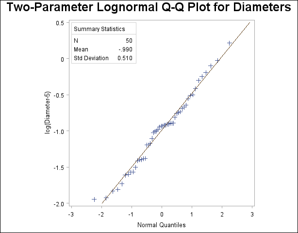
Because the point pattern in Output 4.33.1 is linear, you can estimate the lognormal parameters
 and
and  as the normal plot estimates of
  and , which are
  0.99 and 0.51. These values correspond to the previous estimates of 0.92 for and 0.5 for from Example 4.31. A sample program for this example, uniex18.sas, is available in the SAS Sample Library for Base SAS software.
 Copyright © SAS Institute, Inc. All Rights Reserved.