Example 4.35 Creating a Cumulative Distribution Plot

A company that produces fiber-optic cord is interested in the breaking strength of the cord. The following statements create a data set named Cord, which contains 50 breaking strengths measured in pounds per square inch (psi):

data Cord;
   label Strength="Breaking Strength (psi)";
   input Strength @@;
datalines;
6.94 6.97 7.11 6.95 7.12 6.70 7.13 7.34 6.90 6.83
7.06 6.89 7.28 6.93 7.05 7.00 7.04 7.21 7.08 7.01
7.05 7.11 7.03 6.98 7.04 7.08 6.87 6.81 7.11 6.74
6.95 7.05 6.98 6.94 7.06 7.12 7.19 7.12 7.01 6.84
6.91 6.89 7.23 6.98 6.93 6.83 6.99 7.00 6.97 7.01
;
run;

You can use the CDFPLOT statement to fit any of six theoretical distributions (beta, exponential, gamma, lognormal, normal, and Weibull) and superimpose them on the cdf plot. The following statements use the NORMAL option to display a fitted normal distribution function on a cdf plot of breaking strengths:

title 'Cumulative Distribution Function of Breaking Strength';
ods graphics on;
proc univariate data=Cord noprint;
   cdf Strength / normal;
   inset normal(mu sigma);
run;

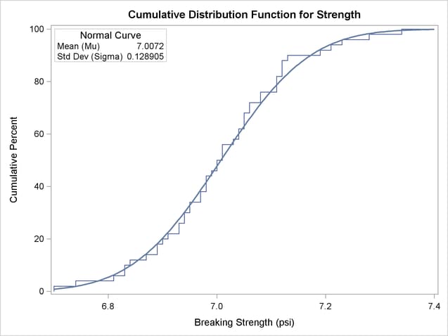
The NORMAL option requests the fitted curve. The INSET statement requests an inset containing the parameters of the fitted curve, which are the sample mean and standard deviation. For more information about the INSET statement, see INSET Statement. The resulting plot is shown in Output 4.35.1.

Output 4.35.1 Cumulative Distribution Function

The plot shows a symmetric distribution with observations concentrated 6.9 and 7.1. The agreement between the empirical and the normal distribution functions in Output 4.35.1 is evidence that the normal distribution is an appropriate model for the distribution of breaking strengths.