The OPTNET Procedure
- Overview
-
Getting Started

-
SyntaxFunctional SummaryPROC OPTNET StatementBICONCOMP StatementCLIQUE StatementCONCOMP StatementCYCLE StatementDATA_LINKS_VAR StatementDATA_MATRIX_VAR StatementDATA_NODES_VAR StatementLINEAR_ASSIGNMENT StatementMINCOSTFLOW StatementMINCUT StatementMINSPANTREE StatementPERFORMANCE StatementSHORTPATH StatementTRANSITIVE_CLOSURE StatementTSP Statement
-
DetailsGraph Input DataMatrix Input DataData Input OrderParallel ProcessingNumeric LimitationsSize LimitationsBiconnected Components and Articulation PointsCliqueConnected ComponentsCycleLinear Assignment (Matching)Minimum-Cost Network FlowMinimum CutMinimum Spanning TreeShortest PathTransitive ClosureTraveling Salesman ProblemMacro VariablesODS Table Names
-
ExamplesArticulation Points in a Terrorist NetworkCycle Detection for Kidney Donor ExchangeLinear Assignment Problem for Minimizing Swim TimesLinear Assignment Problem, Sparse Format versus Dense FormatMinimum Spanning Tree for Computer Network TopologyTransitive Closure for Identification of Circular Dependencies in a Bug Tracking SystemTraveling Salesman Tour through US Capital Cities
- References
Traveling Salesman Problem
The traveling salesman problem (TSP) finds a minimum-cost tour in a graph, G, that has a node set, N, and a link set, A. A path in a graph is a sequence of nodes, each of which has a link to the next node in the sequence. An elementary cycle is a path in which the start node and end node are the same and no node appears more than once in the sequence. A Hamiltonian cycle (or tour) is an elementary cycle that visits every node. In solving the TSP, then, the goal is to find a Hamiltonian cycle of minimum
total cost, where the total cost is the sum of the costs of the links in the tour. Associated with each link  are a binary variable
  , which indicates whether link is part of the tour, and a cost
  . Let
. Let  . Then an integer linear programming formulation of the TSP (for an undirected graph G) is as follows:
![\[ \begin{array}{llllll} \text {minimize} & \displaystyle \sum _{(i,j) \in A} c_{ij} x_{ij} \\ \text {subject to} & \displaystyle \sum _{(i,j) \in \delta ({i})} x_{i,j} & = & 2 & i \in N & (\mr{two\_ match}) \\ & \displaystyle \sum _{(i,j) \in \delta (S)}x_{ij} & \geq & 2 & S \subset N, \; 2 \leq |S| \leq |N| - 1 & (\mr{subtour\_ elim})\\ & x_{ij} \in \{ 0,1\} & & & (i,j) \in A \end{array} \]](images/ornoaug_optnet0077.png)
The equations (two_match) are the matching constraints, which ensure that each node has degree two in the subgraph. The inequalities (subtour_elim) are the subtour elimination constraints (SECs), which enforce connectivity.
For a directed graph, G, the same formulation and solution approach is used on an expanded graph  , as described in Kumar and Li (1994). PROC OPTNET takes care of the construction of the expanded graph and returns the solution in terms of the original input
graph.
, as described in Kumar and Li (1994). PROC OPTNET takes care of the construction of the expanded graph and returns the solution in terms of the original input
graph.
In practical terms, you can think of the TSP in the context of a routing problem in which each node is a city and the links are roads that connect those cities. If you know the distance between each pair of cities, the goal is to find the shortest possible route that visits each city exactly once. The TSP has applications in planning, logistics, manufacturing, genomics, and many other areas.
In PROC OPTNET, you can invoke the traveling salesman problem solver by using the TSP statement. The options for this statement are described in the section TSP Statement.
The traveling salesman problem solver reports status information in a macro variable called _OROPTNET_TSP_. For more information about this macro variable, see the section Macro Variable _OROPTNET_TSP_.
The algorithm that PROC OPTNET uses for solving the TSP is based on a variant of the branch-and-cut process described in Applegate et al. (2006).
The resulting tour is represented in two ways: in the data set that you specify in the OUT_NODES= option in the PROC OPTNET statement, the tour is specified as a sequence of nodes; in the data set that you specify in the OUT= option of the TSP statement, the tour is specified as a list of links in the optimal tour.
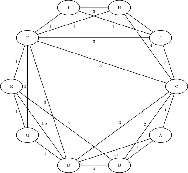
Traveling Salesman Problem Applied to a Simple Undirected Graph
As a simple example, consider the weighted undirected graph in Figure 2.69.
Figure 2.69: A Simple Undirected Graph
You can represent the links data set as follows:
data LinkSetIn;
   input from $ to $ weight @@;
   datalines;
A B 1.0 A C 1.0 A D 1.5 B C 2.0 B D 4.0
B E 3.0 C D 3.0 C F 3.0 C H 4.0 D E 1.5
D F 3.0 D G 4.0 E F 1.0 E G 1.0 F G 2.0
F H 4.0 H I 3.0 I J 1.0 C J 5.0 F J 3.0
F I 1.0 H J 1.0
;
The following statements calculate an optimal traveling salesman tour and output the results in the data sets TSPTour and NodeSetOut:
proc optnet
   loglevel   = moderate
   data_links = LinkSetIn
   out_nodes  = NodeSetOut;
   tsp
      out     = TSPTour;
run;
%put &_OROPTNET_;
%put &_OROPTNET_TSP_;
The progress of the OPTNET procedure is shown in Figure 2.70.
Figure 2.70: PROC OPTNET Log: Optimal Traveling Salesman Tour of a Simple Undirected Graph
| NOTE: ------------------------------------------------------------------------------------------ |
| NOTE: ------------------------------------------------------------------------------------------ |
| NOTE: Running OPTNET version 14.1. |
| NOTE: ------------------------------------------------------------------------------------------ |
| NOTE: ------------------------------------------------------------------------------------------ |
| NOTE: The OPTNET procedure is executing in single-machine mode. |
| NOTE: ------------------------------------------------------------------------------------------ |
| NOTE: ------------------------------------------------------------------------------------------ |
| NOTE: Reading the links data set. |
| NOTE: There were 22 observations read from the data set WORK.LINKSETIN. |
| NOTE: Data input used 0.01 (cpu: 0.00) seconds. |
| NOTE: Building the input graph storage used 0.00 (cpu: 0.00) seconds. |
| NOTE: The input graph storage is using 0.0 MBs (peak: 0.0 MBs) of memory. |
| NOTE: The number of nodes in the input graph is 10. |
| NOTE: The number of links in the input graph is 22. |
| NOTE: ------------------------------------------------------------------------------------------ |
| NOTE: ------------------------------------------------------------------------------------------ |
| NOTE: Processing the traveling salesman problem. |
| NOTE: The initial TSP heuristics found a tour with cost 16 using 0.00 (cpu: 0.00) seconds. |
| NOTE: The MILP presolver value NONE is applied. |
| NOTE: The MILP solver is called. |
| NOTE: The Branch and Cut algorithm is used. |
| Node Active Sols BestInteger BestBound Gap Time |
| 0 1 1 16.0000000 15.5005000 3.22% 0 |
| 0 0 1 16.0000000 16.0000000 0.00% 0 |
| NOTE: Objective = 16. |
| NOTE: Processing the traveling salesman problem used 0.01 (cpu: 0.00) seconds. |
| NOTE: ------------------------------------------------------------------------------------------ |
| NOTE: ------------------------------------------------------------------------------------------ |
| NOTE: Creating nodes data set output. |
| NOTE: Creating traveling salesman data set output. |
| NOTE: Data output used 0.00 (cpu: 0.00) seconds. |
| NOTE: ------------------------------------------------------------------------------------------ |
| NOTE: ------------------------------------------------------------------------------------------ |
| NOTE: The data set WORK.NODESETOUT has 10 observations and 2 variables. |
| NOTE: The data set WORK.TSPTOUR has 10 observations and 3 variables. |
| STATUS=OK TSP=OPTIMAL |
| STATUS=OPTIMAL OBJECTIVE=16 RELATIVE_GAP=0 ABSOLUTE_GAP=0 PRIMAL_INFEASIBILITY=0 |
| BOUND_INFEASIBILITY=0 INTEGER_INFEASIBILITY=0 BEST_BOUND=16 NODES=1 ITERATIONS=17 |
| CPU_TIME=0.00 REAL_TIME=0.01 |
The data set NodeSetOut now contains a sequence of nodes in the optimal tour and is shown in Figure 2.71.
Figure 2.71: Nodes in the Optimal Traveling Salesman Tour
The data set TSPTour now contains the links in the optimal tour and is shown in Figure 2.72.
Figure 2.72: Links in the Optimal Traveling Salesman Tour
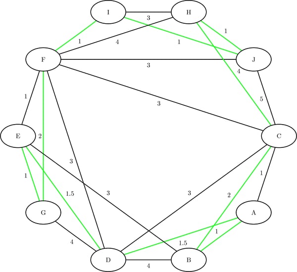
The minimum-cost links are shown in green in Figure 2.73.
Figure 2.73: Optimal Traveling Salesman Tour
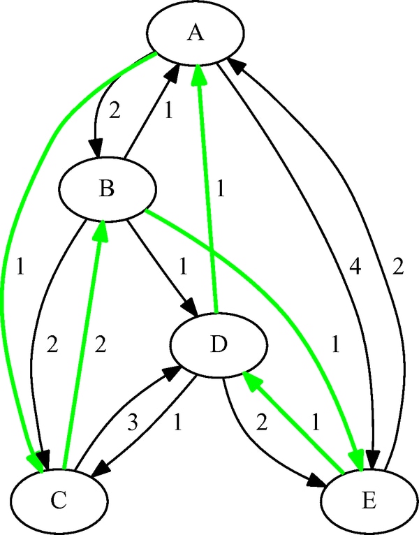
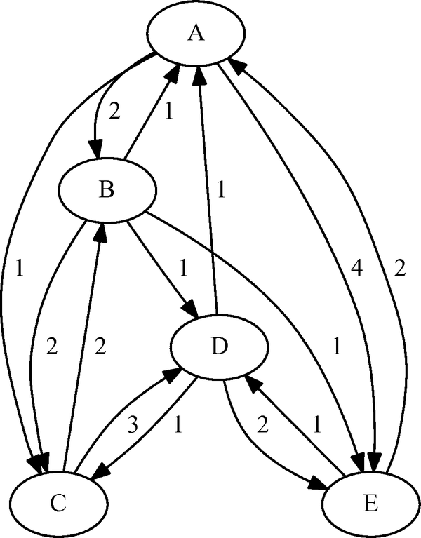
Traveling Salesman Problem Applied to a Simple Directed Graph
As another simple example, consider the weighted directed graph in Figure 2.74.
Figure 2.74: A Simple Directed Graph
You can represent the links data set as follows:
data LinkSetIn;
   input from $ to $ weight @@;
   datalines;
A B 2.0 A C 1.0 A E 4.0 B A 1.0 B C 2.0
B D 1.0 B E 1.0 C B 2.0 C D 3.0 D A 1.0
D C 1.0 D E 2.0 E A 2.0 E D 1.0
;
The following statements calculate an optimal traveling salesman tour (on a directed graph) and output the results in the
data sets TSPTour and NodeSetOut:
proc optnet
   direction  = directed
   loglevel   = moderate
   data_links = LinkSetIn
   out_nodes  = NodeSetOut;
   tsp
      out     = TSPTour;
run;
%put &_OROPTNET_;
%put &_OROPTNET_TSP_;
The progress of the OPTNET procedure is shown in Figure 2.75.
Figure 2.75: PROC OPTNET Log: Optimal Traveling Salesman Tour of a Simple Directed Graph
| NOTE: ------------------------------------------------------------------------------------------ |
| NOTE: ------------------------------------------------------------------------------------------ |
| NOTE: Running OPTNET version 14.1. |
| NOTE: ------------------------------------------------------------------------------------------ |
| NOTE: ------------------------------------------------------------------------------------------ |
| NOTE: The OPTNET procedure is executing in single-machine mode. |
| NOTE: ------------------------------------------------------------------------------------------ |
| NOTE: ------------------------------------------------------------------------------------------ |
| NOTE: Reading the links data set. |
| NOTE: There were 14 observations read from the data set WORK.LINKSETIN. |
| NOTE: Data input used 0.00 (cpu: 0.00) seconds. |
| NOTE: Building the input graph storage used 0.00 (cpu: 0.00) seconds. |
| NOTE: The input graph storage is using 0.0 MBs (peak: 0.0 MBs) of memory. |
| NOTE: The number of nodes in the input graph is 5. |
| NOTE: The number of links in the input graph is 14. |
| NOTE: ------------------------------------------------------------------------------------------ |
| NOTE: ------------------------------------------------------------------------------------------ |
| NOTE: The TSP solver is starting using an augmented symmetric graph with 10 nodes and 19 links. |
| NOTE: ------------------------------------------------------------------------------------------ |
| NOTE: ------------------------------------------------------------------------------------------ |
| NOTE: Processing the traveling salesman problem. |
| NOTE: The initial TSP heuristics found a tour with cost 6 using 0.00 (cpu: 0.00) seconds. |
| NOTE: The MILP presolver value NONE is applied. |
| NOTE: The MILP solver is called. |
| NOTE: The Branch and Cut algorithm is used. |
| Node Active Sols BestInteger BestBound Gap Time |
| 0 1 1 6.0000000 5.9001000 1.69% 0 |
| 0 0 1 6.0000000 6.0000000 0.00% 0 |
| NOTE: Objective = 6. |
| NOTE: Processing the traveling salesman problem used 0.00 (cpu: 0.00) seconds. |
| NOTE: ------------------------------------------------------------------------------------------ |
| NOTE: ------------------------------------------------------------------------------------------ |
| NOTE: Creating nodes data set output. |
| NOTE: Creating traveling salesman data set output. |
| NOTE: Data output used 0.00 (cpu: 0.02) seconds. |
| NOTE: ------------------------------------------------------------------------------------------ |
| NOTE: ------------------------------------------------------------------------------------------ |
| NOTE: The data set WORK.NODESETOUT has 5 observations and 2 variables. |
| NOTE: The data set WORK.TSPTOUR has 5 observations and 3 variables. |
| STATUS=OK TSP=OPTIMAL |
| STATUS=OPTIMAL OBJECTIVE=6 RELATIVE_GAP=2.96E-16 ABSOLUTE_GAP=-1.77636E-15 |
| PRIMAL_INFEASIBILITY=0 BOUND_INFEASIBILITY=0 INTEGER_INFEASIBILITY=0 BEST_BOUND=6 NODES=1 |
| ITERATIONS=8 CPU_TIME=0.00 REAL_TIME=0.00 |
The data set NodeSetOut now contains a sequence of nodes in the optimal tour and is shown in Figure 2.76.
The data set TSPTour now contains the links in the optimal tour and is shown in Figure 2.77.
Figure 2.77: Links in the Optimal Traveling Salesman Tour
The minimum-cost links are shown in green in Figure 2.78.
Figure 2.78: Optimal Traveling Salesman Tour