The OPTNET Procedure

Minimum-Cost Network Flow

Subsections:

Minimum-Cost Network Flow for a Simple Directed Graph
Minimum-Cost Network Flow with Flexible Supply and Demand

The minimum-cost network flow (MCF) problem is a fundamental problem in network analysis that involves sending flow over a network at minimal cost. Let $G=(N,A)$ be a directed graph. For each link $(i,j) \in A$ , associate a cost per unit of flow, designated as $c_{ij}$ . The demand (or supply) at each node $i \in N$ is designated as $b_ i$ , where $b_ i \geq 0$ denotes a supply node and $b_ i < 0$ denotes a demand node. These values must be within $[b_ i^ l, b_ i^ u]$ . Define decision variables $x_{ij}$ that denote the amount of flow sent from node i to node j. The amount of flow that can be sent across each link is bounded to be within $[l_{ij}, u_{ij}]$ . The problem can be modeled as a linear programming problem as follows:

$\begin{alignat*}{3}& \text {minimize} & & \quad \sum _{(i,j) \in A} c_{ij} x_{ij} \\ & \text {subject to} & & \quad b_ i^ l \leq \sum _{(i,j) \in A} x_{ij} - \sum _{(j,i) \in A} x_{ji} \leq b^ u_ i & & \quad i \in N\\ & & & \quad l_{ij} \le x_{ij} \le u_{ij} & & \quad (i,j) \in A \end{alignat*}$

When $b_ i=b_ i^ l=b_ i^ u$ for all nodes $i \in N$ , the problem is called a pure network flow problem. For these problems, the sum of the supplies and demands must be equal to 0 to ensure that a feasible solution exists.

In PROC OPTNET, you can invoke the minimum-cost network flow solver by using the MINCOSTFLOW statement. The options for this statement are described in the section MINCOSTFLOW Statement.

The minimum-cost network flow solver reports status information in a macro variable called _OROPTNET_MCF_. For more information about this macro variable, see the section Macro Variable _OROPTNET_MCF_.

The algorithm that PROC OPTNET uses to solve the MCF problem is a variant of the primal network simplex algorithm (Ahuja, Magnanti, and Orlin 1993). Sometimes the directed graph G is disconnected. In this case, the problem is first decomposed into its weakly connected components, and then each minimum-cost flow problem is solved separately.

The input for the network is the standard graph input, which is described in the section Graph Input Data. The links data set, which is specified in the DATA_LINKS= option in the PROC OPTNET statement, contains the following columns:

weight, which defines the link cost $c_{ij}$
lower, which defines the link lower bound $l_{ij}$ . The default is 0.
upper, which defines the link upper bound $u_{ij}$ . The default is $\infty$ .

The nodes data set, which is specified in the DATA_NODES= option in the PROC OPTNET statement, can contain the following columns:

weight, which defines the node supply lower bound $b_ i^ l$ . The default is 0.
weight2, which defines the node supply upper bound $b_ i^ u$ . The default is $\infty$ .

To define a pure network in which the node supply must be met exactly, use the weight variable only. You do not need to specify all the node supply bounds. For any missing node, the solver uses a lower and upper bound of 0.

To explicitly define an upper bound of $\infty$ , use the special missing value, (.I). To explicitly define a lower bound of $-\infty$ , use the special missing value, (.M). Related to infinite bounds, the following scenarios are not supported:

The flow on a link must be bounded from below ( $l_{ij} = -\infty$ is not allowed).
Flow balance constraints cannot be free ( $b_ i^ l = -\infty$ and $b_ i^ u = \infty$ is not allowed).

The resulting optimal flow through the network is written to the links output data set, which is specified in the OUT_LINKS= option in the PROC OPTNET statement.

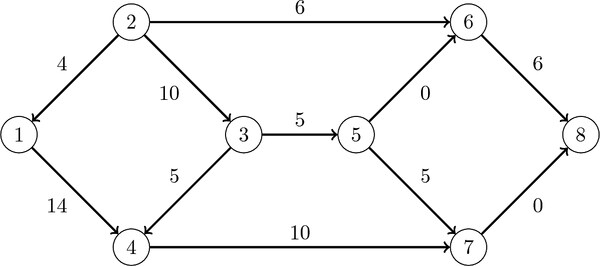
Minimum-Cost Network Flow for a Simple Directed Graph

This example demonstrates how to use the network simplex algorithm to find a minimum-cost flow in a directed graph. Consider the directed graph in Figure 2.39, which appears in Ahuja, Magnanti, and Orlin (1993).

Figure 2.39: Minimum-Cost Network Flow Problem: Data

The directed graph G can be represented by the following links data set LinkSetIn and nodes data set NodeSetIn:

data LinkSetIn;
   input from to weight upper;
   datalines;
1 4 2 15
2 1 1 10
2 3 0 10
2 6 6 10
3 4 1  5
3 5 4 10
4 7 5 10
5 6 2 20
5 7 7 15
6 8 8 10
7 8 9 15
;

data NodeSetIn;
   input node weight;
   datalines;
1  10
2  20
4  -5
7 -15
8 -10
;

You can use the following call to PROC OPTNET to find a minimum-cost flow:

proc optnet
   loglevel        = moderate
   graph_direction = directed
   data_links      = LinkSetIn
   data_nodes      = NodeSetIn
   out_links       = LinkSetOut;
   mincostflow
      logfreq      = 1;
run;
%put &_OROPTNET_;
%put &_OROPTNET_MCF_;

The progress of the procedure is shown in Figure 2.40.

Figure 2.40: PROC OPTNET Log for Minimum-Cost Network Flow

NOTE: ------------------------------------------------------------------------------------------

NOTE: Running OPTNET version 14.1.

NOTE: ------------------------------------------------------------------------------------------

NOTE: The OPTNET procedure is executing in single-machine mode.

NOTE: ------------------------------------------------------------------------------------------

NOTE: Reading the nodes data set.

NOTE: There were 5 observations read from the data set WORK.NODESETIN.

NOTE: Reading the links data set.

NOTE: There were 11 observations read from the data set WORK.LINKSETIN.

NOTE: Data input used 0.00 (cpu: 0.02) seconds.

NOTE: Building the input graph storage used 0.00 (cpu: 0.00) seconds.

NOTE: The input graph storage is using 0.0 MBs (peak: 0.0 MBs) of memory.

NOTE: The number of nodes in the input graph is 8.

NOTE: The number of links in the input graph is 11.

NOTE: ------------------------------------------------------------------------------------------

NOTE: Processing the minimum-cost network flow problem.

NOTE: The network has 1 connected component.

Primal Primal Dual

Iteration Objective Infeasibility Infeasibility Time

1 0.000000E+00 2.000000E+01 8.900000E+01 0.00

2 0.000000E+00 2.000000E+01 8.900000E+01 0.00

3 5.000000E+00 1.500000E+01 8.400000E+01 0.00

4 5.000000E+00 1.500000E+01 8.300000E+01 0.00

5 5.000000E+00 1.500000E+01 8.300000E+01 0.00

6 7.500000E+01 1.500000E+01 7.900000E+01 0.00

7 1.300000E+02 1.000000E+01 7.600000E+01 0.00

8 1.300000E+02 1.000000E+01 7.600000E+01 0.00

9 1.300000E+02 1.000000E+01 7.600000E+01 0.00

10 2.700000E+02 0.000000E+00 0.000000E+00 0.00

NOTE: The Network Simplex solve time is 0.00 seconds.

NOTE: Objective = 270.

NOTE: Processing the minimum-cost network flow problem used 0.00 (cpu: 0.00) seconds.

NOTE: ------------------------------------------------------------------------------------------

NOTE: Creating links data set output.

NOTE: Data output used 0.00 (cpu: 0.00) seconds.

NOTE: ------------------------------------------------------------------------------------------

NOTE: The data set WORK.LINKSETOUT has 11 observations and 5 variables.

STATUS=OK MCF=OPTIMAL

STATUS=OPTIMAL OBJECTIVE=270 CPU_TIME=0.00 REAL_TIME=0.00

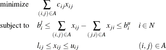
The optimal solution is displayed in Figure 2.41.

Figure 2.41: Minimum-Cost Network Flow Problem: Optimal Solution

Obs	from	to	upper	weight	mcf_flow
1	1	4	15	2	10
2	2	1	10	1	0
3	2	3	10	0	10
4	2	6	10	6	10
5	3	4	5	1	5
6	3	5	10	4	5
7	4	7	10	5	10
8	5	6	20	2	0
9	5	7	15	7	5
10	6	8	10	8	10
11	7	8	15	9	0

The optimal solution is represented graphically in Figure 2.42.

Figure 2.42: Minimum-Cost Network Flow Problem: Optimal Solution

Minimum-Cost Network Flow with Flexible Supply and Demand

Using the same directed graph shown in Figure 2.39, this example demonstrates a network that has a flexible supply and demand. Consider the following adjustments to the node bounds:

Node 1 has an infinite supply, but it still requires at least 10 units to be sent.
Node 4 is a throughput node that can now handle an infinite amount of demand.
Node 8 has a flexible demand. It requires between 6 and 10 units.

You use the special missing values (.I) to represent infinity and (.M) to represent minus infinity. The adjusted node bounds can be represented by the following nodes data set:

data NodeSetIn;
   input node weight weight2;
   datalines;
1  10  .I
2  20  20
4  .M  -5
7 -15 -15
8 -10  -6
;

You can use the following call to PROC OPTNET to find a minimum-cost flow:

proc optnet
   loglevel        = moderate
   graph_direction = directed
   data_links      = LinkSetIn
   data_nodes      = NodeSetIn
   out_links       = LinkSetOut;
   mincostflow
      logfreq      = 1;
run;
%put &_OROPTNET_;
%put &_OROPTNET_MCF_;

The progress of the procedure is shown in Figure 2.43.

Figure 2.43: PROC OPTNET Log for Minimum-Cost Network Flow

NOTE: ------------------------------------------------------------------------------------------

NOTE: Running OPTNET version 14.1.

NOTE: ------------------------------------------------------------------------------------------

NOTE: The OPTNET procedure is executing in single-machine mode.

NOTE: ------------------------------------------------------------------------------------------

NOTE: Reading the nodes data set.

NOTE: There were 5 observations read from the data set WORK.NODESETIN.

NOTE: Reading the links data set.

NOTE: There were 11 observations read from the data set WORK.LINKSETIN.

NOTE: Data input used 0.00 (cpu: 0.00) seconds.

NOTE: Building the input graph storage used 0.00 (cpu: 0.00) seconds.

NOTE: The input graph storage is using 0.0 MBs (peak: 0.0 MBs) of memory.

NOTE: The number of nodes in the input graph is 8.

NOTE: The number of links in the input graph is 11.

NOTE: ------------------------------------------------------------------------------------------

NOTE: Processing the minimum-cost network flow problem.

NOTE: The network has 1 connected component.

Primal Primal Dual

Iteration Objective Infeasibility Infeasibility Time

1 1.000000E+01 2.000000E+01 1.730000E+02 0.00

2 1.000000E+01 2.000000E+01 1.730000E+02 0.00

3 4.500000E+01 2.000000E+01 1.740000E+02 0.00

4 4.500000E+01 2.000000E+01 1.740000E+02 0.00

5 7.500000E+01 1.500000E+01 1.660000E+02 0.00

6 7.500000E+01 1.500000E+01 1.660000E+02 0.00

7 1.590000E+02 9.000000E+00 8.700000E+01 0.00

8 1.590000E+02 9.000000E+00 1.690000E+02 0.00

9 2.140000E+02 4.000000E+00 8.700000E+01 0.00

10 2.140000E+02 4.000000E+00 8.700000E+01 0.00

11 2.260000E+02 0.000000E+00 0.000000E+00 0.00

12 2.260000E+02 0.000000E+00 0.000000E+00 0.00

13 2.260000E+02 0.000000E+00 0.000000E+00 0.00

14 2.260000E+02 0.000000E+00 0.000000E+00 0.00

NOTE: The Network Simplex solve time is 0.00 seconds.

NOTE: Objective = 226.

NOTE: Processing the minimum-cost network flow problem used 0.00 (cpu: 0.00) seconds.

NOTE: ------------------------------------------------------------------------------------------

NOTE: Creating links data set output.

NOTE: Data output used 0.00 (cpu: 0.00) seconds.

NOTE: ------------------------------------------------------------------------------------------

NOTE: The data set WORK.LINKSETOUT has 11 observations and 5 variables.

STATUS=OK MCF=OPTIMAL

STATUS=OPTIMAL OBJECTIVE=226 CPU_TIME=0.00 REAL_TIME=0.00

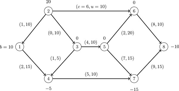
The optimal solution is displayed in Figure 2.44.

Figure 2.44: Minimum-Cost Network Flow Problem: Optimal Solution

Obs	from	to	upper	weight	mcf_flow
1	1	4	15	2	14
2	2	1	10	1	4
3	2	3	10	0	10
4	2	6	10	6	6
5	3	4	5	1	5
6	3	5	10	4	5
7	4	7	10	5	10
8	5	6	20	2	0
9	5	7	15	7	5
10	6	8	10	8	6
11	7	8	15	9	0

The optimal solution is represented graphically in Figure 2.45.

Figure 2.45: Minimum-Cost Network Flow Problem: Optimal Solution

Obs	from	to	upper	weight	mcf_flow
1	1	4	15	2	10
2	2	1	10	1	0
3	2	3	10	0	10
4	2	6	10	6	10
5	3	4	5	1	5
6	3	5	10	4	5
7	4	7	10	5	10
8	5	6	20	2	0
9	5	7	15	7	5
10	6	8	10	8	10
11	7	8	15	9	0

Obs	from	to	upper	weight	mcf_flow
1	1	4	15	2	14
2	2	1	10	1	4
3	2	3	10	0	10
4	2	6	10	6	6
5	3	4	5	1	5
6	3	5	10	4	5
7	4	7	10	5	10
8	5	6	20	2	0
9	5	7	15	7	5
10	6	8	10	8	6
11	7	8	15	9	0

Obs	from	to	upper	weight	mcf_flow
1	1	4	15	2	10
2	2	1	10	1	0
3	2	3	10	0	10
4	2	6	10	6	10
5	3	4	5	1	5
6	3	5	10	4	5
7	4	7	10	5	10
8	5	6	20	2	0
9	5	7	15	7	5
10	6	8	10	8	10
11	7	8	15	9	0

Obs	from	to	upper	weight	mcf_flow
1	1	4	15	2	14
2	2	1	10	1	4
3	2	3	10	0	10
4	2	6	10	6	6
5	3	4	5	1	5
6	3	5	10	4	5
7	4	7	10	5	10
8	5	6	20	2	0
9	5	7	15	7	5
10	6	8	10	8	6
11	7	8	15	9	0

Obs	from	to	upper	weight	mcf_flow
1	1	4	15	2	10
2	2	1	10	1	0
3	2	3	10	0	10
4	2	6	10	6	10
5	3	4	5	1	5
6	3	5	10	4	5
7	4	7	10	5	10
8	5	6	20	2	0
9	5	7	15	7	5
10	6	8	10	8	10
11	7	8	15	9	0

Obs	from	to	upper	weight	mcf_flow
1	1	4	15	2	14
2	2	1	10	1	4
3	2	3	10	0	10
4	2	6	10	6	6
5	3	4	5	1	5
6	3	5	10	4	5
7	4	7	10	5	10
8	5	6	20	2	0
9	5	7	15	7	5
10	6	8	10	8	6
11	7	8	15	9	0