The Network Solver
- Overview
- Getting Started
-
Syntax

-
DetailsInput Data for the Network SolverSolving over Subsets of Nodes and Links (Filters)Numeric LimitationsBiconnected Components and Articulation PointsCliqueConnected ComponentsCycleLinear Assignment (Matching)Minimum-Cost Network FlowMinimum CutMinimum Spanning TreeShortest PathTransitive ClosureTraveling Salesman ProblemMacro Variable _OROPTMODEL_
-
ExamplesArticulation Points in a Terrorist NetworkCycle Detection for Kidney Donor ExchangeLinear Assignment Problem for Minimizing Swim TimesLinear Assignment Problem, Sparse Format versus Dense FormatMinimum Spanning Tree for Computer Network TopologyTransitive Closure for Identification of Circular Dependencies in a Bug Tracking SystemTraveling Salesman Tour through US Capital Cities
- References
Minimum-Cost Network Flow
The minimum-cost network flow problem (MCF) is a fundamental problem in network analysis that involves sending flow over a network at minimal cost. Let  be a directed graph. For each link
  , associate a cost per unit of flow, designated by
  . The demand (or supply) at each node
  is designated as
  , where
  denotes a supply node and
  denotes a demand node. These values must be within
 ![$[b_ i^ l, b_ i^ u]$](images/ormpug_networksolver0061.png) . Define decision variables
. Define decision variables  that denote the amount of flow sent from node i to node j. The amount of flow that can be sent across each link is bounded to be within
 ![$[l_{ij}, u_{ij}]$](images/ormpug_networksolver0063.png) . The problem can be modeled as a linear programming problem as follows:
. The problem can be modeled as a linear programming problem as follows:
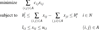
When  for all nodes , the problem is called a pure network flow problem. For these problems, the sum of the supplies and demands must be equal to 0 to ensure that a feasible solution exists.
In the network solver, you can invoke the minimum-cost network flow solver by using the MINCOSTFLOW option.
The algorithm that the network solver uses for solving MCF is a variant of the primal network simplex algorithm (Ahuja, Magnanti, and Orlin 1993). Sometimes the directed graph G is disconnected. In this case, the problem is first decomposed into its weakly connected components, and then each minimum-cost flow problem is solved separately.
The input for the network is the standard graph input, which is described in the section Input Data for the Network Solver. The MCF option uses the following suboptions of the LINKS= input option that specify link-indexed numeric arrays:
-
The WEIGHT= suboption defines the link cost
per unit of flow. (The default is 0, but if the WEIGHT= suboption is not specified, then the default is 1.)
-
The LOWER= suboption defines the link flow lower bound
 . (The default is 0.)
-
The UPPER= suboption defines the link flow upper bound
 . (The default is
  .)
.)
The MCF option uses the WEIGHT= suboption of the NODES= option to specify supply. The parameter is a numeric array that is positive for supply nodes and negative for demand nodes.
The resulting optimal flow through the network is written to the link-indexed numeric array that is specified in the FLOW= suboption of the OUT= option in the SOLVE WITH NETWORK statement.
Minimum Cost Network Flow for a Simple Directed Graph
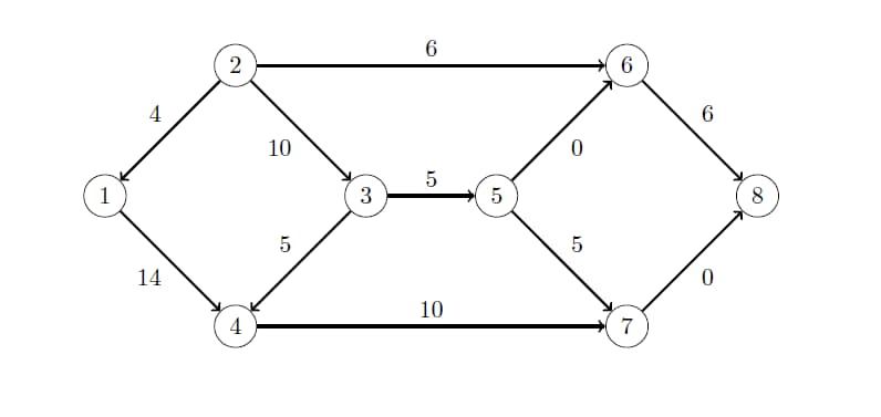
The following example demonstrates how to use the network simplex algorithm to find a minimum-cost flow in a directed graph. Consider the directed graph in Figure 9.38, which appears in Ahuja, Magnanti, and Orlin (1993).
Figure 9.38: Minimum-Cost Network Flow Problem: Data
The directed graph G can be represented by the following links data set LinkSetIn and nodes data set NodeSetIn:
data LinkSetIn;
   input from to weight upper;
   datalines;
1 4 2 15
2 1 1 10
2 3 0 10
2 6 6 10
3 4 1  5
3 5 4 10
4 7 5 10
5 6 2 20
5 7 7 15
6 8 8 10
7 8 9 15
;
data NodeSetIn;
   input node weight;
   datalines;
1  10
2  20
4  -5
7 -15
8 -10
;
You can use the following call to the network solver to find a minimum-cost flow:
proc optmodel;
   set <num,num> LINKS;
   num cost{LINKS};
   num upper{LINKS};
   read data LinkSetIn into LINKS=[from to] cost=weight upper;
   set NODES = union {<i,j> in LINKS} {i,j};
   num supply{NODES} init 0;
   read data NodeSetIn into [node] supply=weight;
   num flow{LINKS};

   solve with network /
      loglevel        = moderate
      logfreq         = 1
      graph_direction = directed
      links           = (upper=upper weight=cost)
      nodes           = (weight=supply)
      mcf
      out             = (flow=flow)
   ;

   print flow;
   create data LinkSetOut from [from to] upper cost flow;
quit;
The progress of the procedure is shown in Figure 9.39.
Figure 9.39: Network Solver Log for Minimum-Cost Network Flow
| NOTE: There were 11 observations read from the data set WORK.LINKSETIN. |
| NOTE: There were 5 observations read from the data set WORK.NODESETIN. |
| NOTE: The number of nodes in the input graph is 8. |
| NOTE: The number of links in the input graph is 11. |
| NOTE: Processing the minimum-cost network flow problem. |
| NOTE: The network has 1 connected component. |
| Primal Primal Dual |
| Iteration Objective Infeasibility Infeasibility Time |
| 1 0.000000E+00 2.000000E+01 8.900000E+01 0.00 |
| 2 0.000000E+00 2.000000E+01 8.900000E+01 0.00 |
| 3 5.000000E+00 1.500000E+01 8.400000E+01 0.00 |
| 4 5.000000E+00 1.500000E+01 8.300000E+01 0.00 |
| 5 7.500000E+01 1.500000E+01 8.300000E+01 0.00 |
| 6 7.500000E+01 1.500000E+01 7.900000E+01 0.00 |
| 7 1.300000E+02 1.000000E+01 7.600000E+01 0.00 |
| 8 2.700000E+02 0.000000E+00 0.000000E+00 0.00 |
| NOTE: The Network Simplex solve time is 0.00 seconds. |
| NOTE: Objective = 270. |
| NOTE: Processing the minimum-cost network flow problem used 0.00 (cpu: 0.00) |
| seconds. |
| NOTE: The data set WORK.LINKSETOUT has 11 observations and 5 variables. |
The optimal solution is displayed in Figure 9.40.
Figure 9.40: Minimum-Cost Network Flow Problem: Optimal Solution
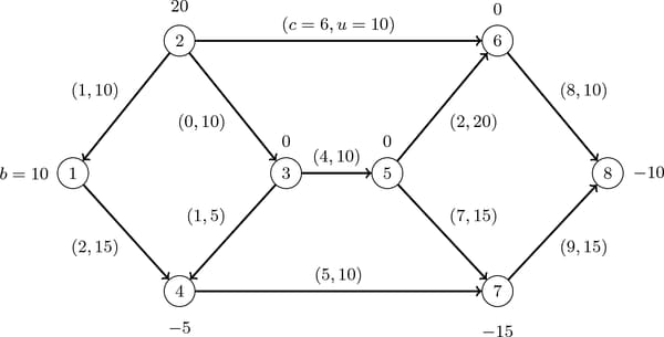
The optimal solution is represented graphically in Figure 9.41.
Figure 9.41: Minimum-Cost Network Flow Problem: Optimal Solution
Minimum-Cost Network Flow with Flexible Supply and Demand
Using the same directed graph shown in Figure 9.38, this example demonstrates a network that has a flexible supply and demand. Consider the following adjustments to the node bounds:
-
Node 1 has an infinite supply, but it still requires at least 10 units to be sent.
-
Node 4 is a throughput node that can now handle an infinite amount of demand.
-
Node 8 has a flexible demand. It requires between 6 and 10 units.
You use the special missing values (.I) to represent infinity and (.M) to represent minus infinity. The adjusted node bounds can be represented by the following nodes data set:
data NodeSetIn;
   input node weight weight2;
   datalines;
1  10  .I
2  20  20
4  .M  -5
7 -15 -15
8 -10  -6
;
You can use the following call to PROC OPTMODEL to find a minimum-cost flow:
proc optmodel;
   set <num,num> LINKS;
   num cost{LINKS};
   num upper{LINKS};
      read data LinkSetIn into LINKS=[from to] cost=weight upper;
   set <num> NODES;
   num supply{NODES};
   num supplyUB{NODES}; /* also demand lower bound, if negative */
      read data NodeSetIn into NODES=[node] supply=weight supplyUB=weight2;
   num flow{LINKS};

   solve with NETWORK /
      direction = directed
      links     = ( upper = upper weight = cost )
      nodes     = ( weight = supply weight2 = supplyUB )
      mcf
      out       = ( flow = flow )
   ;
   print flow;
   create data LinkSetOut from [from to] upper cost flow;
quit;
The progress of the procedure is shown in Figure 9.42.
Figure 9.42: PROC OPTMODEL Log for Minimum-Cost Network Flow
| NOTE: There were 11 observations read from the data set WORK.LINKSETIN. |
| NOTE: There were 5 observations read from the data set WORK.NODESETIN. |
| NOTE: The number of nodes in the input graph is 8. |
| NOTE: The number of links in the input graph is 11. |
| NOTE: Processing the minimum-cost network flow problem. |
| NOTE: Objective = 226. |
| NOTE: Processing the minimum-cost network flow problem used 0.00 (cpu: 0.00) |
| seconds. |
| NOTE: The data set WORK.LINKSETOUT has 11 observations and 5 variables. |
The optimal solution is displayed in Figure 9.43.
Figure 9.43: Minimum-Cost Network Flow Problem: Optimal Solution
The optimal solution is represented graphically in Figure 9.44.
Figure 9.44: Minimum-Cost Network Flow Problem: Optimal Solution