The Network Solver

Cycle

Subsections:

Cycle Detection of a Simple Directed Graph

A path in a graph is a sequence of nodes, each of which has a link to the next node in the sequence. An elementary cycle is a path in which the start node and end node are the same and otherwise no node appears more than once in the sequence.

In the network solver, you can find you can find (or just count) the elementary cycles of an input graph by invoking the CYCLE= algorithm option. To find the cycles and report them in a set, use the CYCLES= suboption in the OUT= option. You do not need to use the CYCLES= suboption to simply count the cycles.

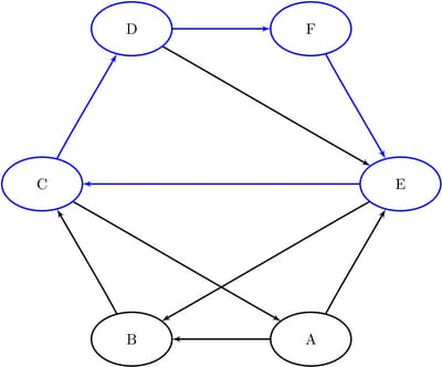
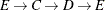
For undirected graphs, each link represents two directed links. For this reason, the following cycles are filtered out: trivial cycles ( $A \rightarrow B \rightarrow A$ ) and duplicate cycles that are found by traversing a cycle in both directions ( $A \rightarrow B \rightarrow C \rightarrow A$ and $A \rightarrow C \rightarrow B \rightarrow A$ ).

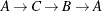The results of the cycle detection algorithm are written to the set that you specify in the CYCLES= suboption in the OUT= option. Each node of each cycle is listed in the CYCLES= set along with a cycle ID (the first argument of the tuple) to identify the cycle to which it belongs. The second argument of the tuple defines the order (sequence) of the node in the cycle.

The algorithm that the network solver uses to compute all cycles is a variant of the algorithm in Johnson (1975). This algorithm runs in time 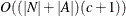$O((|N|+|A|)(c+1))$ , where c is the number of elementary cycles in the graph. So the algorithm should scale to large graphs that contain few cycles. However, some graphs can have a very large number of cycles, so the algorithm might not scale.

If MODE=ALL_CYCLES and there are many cycles, the CYCLES= set can become very large. It might be beneficial to check the number of cycles before you try to create the CYCLES= set. When you specify MODE=FIRST_CYCLE, the algorithm returns the first cycle that it finds and stops processing. This should run relatively quickly. For large-scale graphs, the MINLINKWEIGHT= and MAXLINKWEIGHT= suboptions might increase the computation time.

Cycle Detection of a Simple Directed Graph

This section provides a simple example of using the cycle detection algorithm on the simple directed graph G that is shown in Figure 9.29. Two other examples are Example 9.2: Cycle Detection for Kidney Donor Exchange, which shows the use of cycle detection for optimizing a kidney donor exchange, and Example 9.6: Transitive Closure for Identification of Circular Dependencies in a Bug Tracking System, which shows an application of cycle detection to dependencies between bug reports.

Figure 9.29: A Simple Directed Graph G

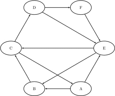
The directed graph G can be represented by the following links data set, LinkSetIn:

data LinkSetIn;
   input from $ to $ @@;
   datalines;
A B  A E  B C  C A  C D
D E  D F  E B  E C  F E
;

The following statements check whether the graph has a cycle:

proc optmodel;
   set<str,str> LINKS;
   read data LinkSetIn into LINKS=[from to];
   set<num,num,str> CYCLES;

   solve with NETWORK /
      graph_direction = directed
      links           = (include=LINKS)
      cycle           = (mode=first_cycle)
   ;
quit;

The result is written to the log of the procedure, as shown in Figure 9.30.

Figure 9.30: Network Solver Log: Check the Existence of a Cycle in a Simple Directed Graph

NOTE: There were 10 observations read from the data set WORK.LINKSETIN.

NOTE: The number of nodes in the input graph is 6.

NOTE: The number of links in the input graph is 10.

NOTE: Processing cycle detection.

NOTE: The graph does have a cycle.

NOTE: Processing cycle detection used 0.00 (cpu: 0.00) seconds.

The following statements count the number of cycles in the graph:

proc optmodel;
   set<str,str> LINKS;
   read data LinkSetIn into LINKS=[from to];
   set<num,num,str> CYCLES;

   solve with NETWORK /
      graph_direction = directed
      links           = (include=LINKS)
      cycle           = (mode=all_cycles)
   ;
quit;

The result is written to the log of the procedure, as shown in Figure 9.31.

Figure 9.31: Network Solver Log: Count the Number of Cycles in a Simple Directed Graph

NOTE: There were 10 observations read from the data set WORK.LINKSETIN.

NOTE: The number of nodes in the input graph is 6.

NOTE: The number of links in the input graph is 10.

NOTE: Processing cycle detection.

NOTE: The graph has 7 cycles.

NOTE: Processing cycle detection used 0.00 (cpu: 0.00) seconds.

The following statements return the first cycle found in the graph:

proc optmodel;
   set<str,str> LINKS;
   read data LinkSetIn into LINKS=[from to];
   set<num,num,str> CYCLES;

   solve with NETWORK /
      graph_direction = directed
      links           = (include=LINKS)
      cycle           = (mode=first_cycle)
      out             = (cycles=CYCLES)
   ;

   put CYCLES;
   create data Cycles from [cycle order node]=CYCLES;
quit;

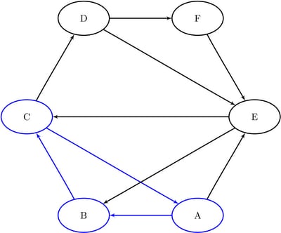
The data set Cycles now contains the first cycle found in the input graph; it is shown in Figure 9.32.

Figure 9.32: First Cycle Found in a Simple Directed Graph

cycle	order	node
1	1	A
1	2	B
1	3	C
1	4	A

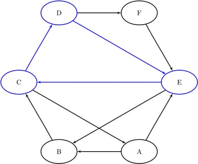
The first cycle that is found in the input graph is shown graphically in Figure 9.33.

Figure 9.33: $A \rightarrow B \rightarrow C \rightarrow A$

The following statements return all the cycles in the graph:

proc optmodel;
   set<str,str> LINKS;
   read data LinkSetIn into LINKS=[from to];
   set<num,num,str> CYCLES;

   solve with NETWORK /
      graph_direction = directed
      links           = (include=LINKS)
      cycle           = (mode=all_cycles)
      out             = (cycles=CYCLES)
   ;

   put CYCLES;
   create data Cycles from [cycle order node]=CYCLES;
quit;

The data set Cycles now contains all the cycles in the input graph; it is shown in Figure 9.34.

Figure 9.34: All Cycles in a Simple Directed Graph

cycle	order	node
1	1	A
1	2	B
1	3	C
1	4	A
2	1	A
2	2	E
2	3	B
2	4	C
2	5	A
3	1	A
3	2	E
3	3	C
3	4	A
4	1	B
4	2	C
4	3	D
4	4	E
4	5	B
5	1	B
5	2	C
5	3	D
5	4	F
5	5	E
5	6	B
6	1	E
6	2	C
6	3	D
6	4	E
7	1	E
7	2	C
7	3	D
7	4	F
7	5	E

The six additional cycles are shown graphically in Figure 9.35 through Figure 9.37.

Figure 9.35: Cycles

$A \rightarrow E \rightarrow B \rightarrow C \rightarrow A$	$A \rightarrow E \rightarrow C \rightarrow A$
$\quad$

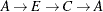
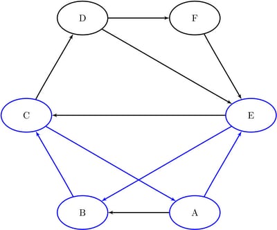
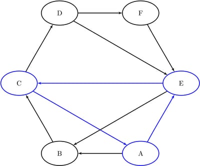
Figure 9.36: Cycles

$B \rightarrow C \rightarrow D \rightarrow E \rightarrow B$	$B \rightarrow C \rightarrow D \rightarrow F \rightarrow E \rightarrow B$
$\quad$

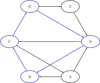
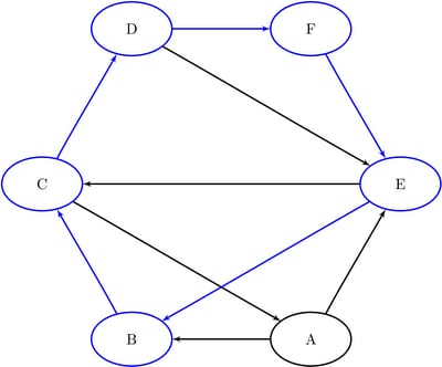
Figure 9.37: Cycles

$E \rightarrow C \rightarrow D \rightarrow E$	$E \rightarrow C \rightarrow D \rightarrow F \rightarrow E$
$\quad$

cycle	order	node
1	1	A
1	2	B
1	3	C
1	4	A
2	1	A
2	2	E
2	3	B
2	4	C
2	5	A
3	1	A
3	2	E
3	3	C
3	4	A
4	1	B
4	2	C
4	3	D
4	4	E
4	5	B
5	1	B
5	2	C
5	3	D
5	4	F
5	5	E
5	6	B
6	1	E
6	2	C
6	3	D
6	4	E
7	1	E
7	2	C
7	3	D
7	4	F
7	5	E

cycle	order	node
1	1	A
1	2	B
1	3	C
1	4	A
2	1	A
2	2	E
2	3	B
2	4	C
2	5	A
3	1	A
3	2	E
3	3	C
3	4	A
4	1	B
4	2	C
4	3	D
4	4	E
4	5	B
5	1	B
5	2	C
5	3	D
5	4	F
5	5	E
5	6	B
6	1	E
6	2	C
6	3	D
6	4	E
7	1	E
7	2	C
7	3	D
7	4	F
7	5	E

cycle	order	node
1	1	A
1	2	B
1	3	C
1	4	A
2	1	A
2	2	E
2	3	B
2	4	C
2	5	A
3	1	A
3	2	E
3	3	C
3	4	A
4	1	B
4	2	C
4	3	D
4	4	E
4	5	B
5	1	B
5	2	C
5	3	D
5	4	F
5	5	E
5	6	B
6	1	E
6	2	C
6	3	D
6	4	E
7	1	E
7	2	C
7	3	D
7	4	F
7	5	E