The Decomposition Algorithm
- Overview
-
Getting Started

-
SyntaxDecomposition Algorithm Options in the PROC OPTLP Statement or the SOLVE WITH LP Statement in PROC OPTMODELDecomposition Algorithm Options in the PROC OPTMILP Statement or the SOLVE WITH MILP Statement in PROC OPTMODELDECOMP StatementDECOMP_MASTER StatementDECOMP_MASTER_IP StatementDECOMP_SUBPROB Statement
-
Details
-
ExamplesMulticommodity Flow ProblemGeneralized Assignment ProblemBlock-Diagonal Structure and METHOD=CONCOMP in Single-Machine ModeBlock-Diagonal Structure and METHOD=CONCOMP in Distributed ModeBlock-Angular Structure and METHOD=AUTOBin Packing ProblemResource Allocation ProblemVehicle Routing ProblemATM Cash Management in Single-Machine ModeATM Cash Management in Distributed ModeKidney Donor Exchange
- References
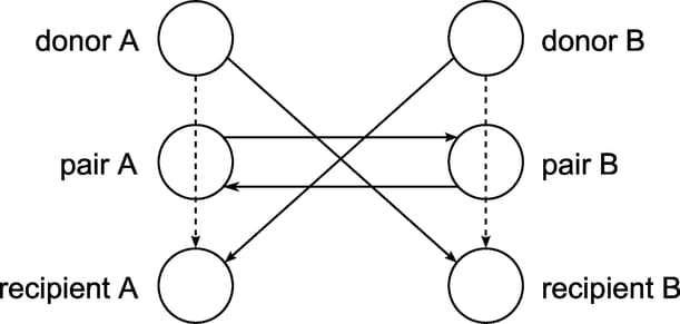
This example looks at an application of integer programming to help create a kidney donor exchange. Suppose someone needs a kidney transplant and a family member is willing to donate a kidney. If the donor and recipient are incompatible (because of conflicting blood types, tissue mismatch, and so on), the transplant cannot proceed. Now suppose two donor-recipient pairs, A and B, are in this same situation, but donor A is compatible with recipient B and donor B is compatible with recipient A. Then two transplants can take place in a two-way swap, which is shown graphically in Figure 15.8.
More generally, an n-way swap that involves n donors and n recipients can be performed (Willingham 2009). To model this problem, define a directed graph as follows. Each node is an incompatible donor-recipient pair. Link ![]() exists if the donor from node i is compatible with the recipient from node j. Let N define the set of nodes and A define the set of arcs. The link weight,
exists if the donor from node i is compatible with the recipient from node j. Let N define the set of nodes and A define the set of arcs. The link weight, ![]() , is a measure of the quality of the match. By introducing dummy links whose weight is 0, you can also include altruistic
donors who have no recipients or recipients who have no donors. The idea is to find a maximum-weight node-disjoint union of
directed cycles. You want the union to be node-disjoint so that no kidney is donated more than once, and you want cycles so
that the donor from node i gives up a kidney if and only if the recipient from node i receives a kidney.
, is a measure of the quality of the match. By introducing dummy links whose weight is 0, you can also include altruistic
donors who have no recipients or recipients who have no donors. The idea is to find a maximum-weight node-disjoint union of
directed cycles. You want the union to be node-disjoint so that no kidney is donated more than once, and you want cycles so
that the donor from node i gives up a kidney if and only if the recipient from node i receives a kidney.
Without any other constraints, the problem could be solved as a linear assignment problem. But doing so would allow arbitrarily
long cycles in the solution. Because of practical considerations (such as travel) and to mitigate risk, each cycle must have
no more than ![]() links. The kidney exchange problem is to find a maximum-weight node-disjoint union of short directed cycles.
links. The kidney exchange problem is to find a maximum-weight node-disjoint union of short directed cycles.
Define an index set ![]() of candidate disjoint unions of short cycles (called matchings). Let
of candidate disjoint unions of short cycles (called matchings). Let ![]() be a binary variable, which, if set to 1, indicates that arc
be a binary variable, which, if set to 1, indicates that arc ![]() is in a matching m. Let
is in a matching m. Let ![]() be a binary variable that, if set to 1, indicates that node i is covered by matching m. In addition, let
be a binary variable that, if set to 1, indicates that node i is covered by matching m. In addition, let ![]() be a binary slack variable that, if set to 1, indicates that node i is not covered by any matching.
be a binary slack variable that, if set to 1, indicates that node i is not covered by any matching.
The kidney donor exchange can be formulated as a MILP as follows:
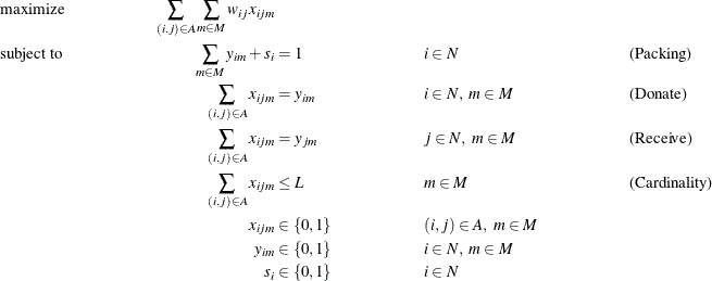
In this formulation, the Packing constraints ensure that each node is covered by at most one matching. The Donate and Receive
constraints enforce the condition that if node i is covered by matching m, then the matching m must use exactly one arc that leaves node i (Donate) and one arc that enters node i (Receive). Conversely, if node i is not covered by matching m, then no arcs that enter or leave node i can be used by matching m. The Cardinality constraints enforce the condition that the number of arcs in matching m must not exceed ![]() .
.
In this formulation, the matching identifier is arbitrary. Because it is not necessary to cover each incompatible donor-recipient pair (node), the Packing constraints can be modeled by using set partitioning constraints and the slack variable s. Consider a decomposition by matching, in which the Packing constraints form the master problem and all other constraints form identical matching subproblems. As described in the section Special Case: Identical Blocks and Ryan-Foster Branching, this is a situation in which an aggregate formulation and Ryan-Foster branching can greatly improve performance by reducing symmetry.
The following DATA step sets up the problem, first creating a random graph on n nodes with link probability p and Uniform(0,1) weight:
/* create random graph on n nodes with arc probability p
   and uniform(0,1) weight */
%let n = 100;
%let p = 0.02;
data ArcData;
   do i = 0 to &n - 1;
      do j = 0 to &n - 1;
         if i eq j then continue;
         else if ranuni(1) < &p then do;
            weight = ranuni(2);
            output;
         end;
      end;
   end;
run;
The following PROC OPTMODEL statements read in the data, declare the optimization model, and use the decomposition algorithm to solve it:
%let max_length = 10;
proc optmodel;
   set <num,num> ARCS;
   num weight {ARCS};
   read data ArcData into ARCS=[i j] weight;
   print weight;
   set NODES = union {<i,j> in ARCS} {i,j};
   set MATCHINGS = 1..card(NODES)/2;

   /* UseNode[i,m] = 1 if node i is used in matching m, 0 otherwise */
   var UseNode {NODES, MATCHINGS} binary;

   /* UseArc[i,j,m] = 1 if arc (i,j) is used in matching m, 0 otherwise */
   var UseArc {ARCS, MATCHINGS} binary;

   /* maximize total weight of arcs used */
   max TotalWeight
      = sum {<i,j> in ARCS, m in MATCHINGS} weight[i,j] * UseArc[i,j,m];

   /* each node appears in at most one matching */
   /* rewrite as set partitioning (so decomp uses identical blocks)
      sum{} x <= 1 => sum{} x + s = 1, s >= 0 with no associated cost */
   var Slack {NODES} binary;
   con Packing {i in NODES}:
      sum {m in MATCHINGS} UseNode[i,m] + Slack[i] = 1;

   /* at most one recipient for each donor */
   con Donate {i in NODES, m in MATCHINGS}:
      sum {<(i),j> in ARCS} UseArc[i,j,m] = UseNode[i,m];

   /* at most one donor for each recipient */
   con Receive {j in NODES, m in MATCHINGS}:
      sum {<i,(j)> in ARCS} UseArc[i,j,m] = UseNode[j,m];

   /* exclude long matchings */
   con Cardinality {m in MATCHINGS}:
      sum {<i,j> in ARCS} UseArc[i,j,m] <= &max_length;

   /* decompose by matching (aggregate formulation) */
   for {i in NODES, m in MATCHINGS} Donate[i,m].block = m;
   for {j in NODES, m in MATCHINGS} Receive[j,m].block = m;
   for {m in MATCHINGS} Cardinality[m].block = m;
   solve with milp / presolver=basic decomp;

   /* save solution to a data set */
   create data Solution from
      [m i j]={m in MATCHINGS, <i,j> in ARCS: UseArc[i,j,m].sol > 0.5}
      weight[i,j];
quit;
In this case, the PRESOLVER=BASIC option ensures that the model maintains its specified symmetry, enabling the algorithm to use the aggregate formulation and Ryan-Foster branching. The solution summary is displayed in Output 15.11.1.
Output 15.11.1: Solution Summary
| Solution Summary | |
|---|---|
| Solver | MILP |
| Algorithm | Decomposition |
| Objective Function | TotalWeight |
| Solution Status | Optimal |
| Objective Value | 26.020287142 |
| Relative Gap | 0 |
| Absolute Gap | 0 |
| Primal Infeasibility | 1.776357E-15 |
| Bound Infeasibility | 2.220446E-16 |
| Integer Infeasibility | 1.554312E-15 |
| Best Bound | 26.020287142 |
| Nodes | 27 |
| Iterations | 151 |
| Presolve Time | 1.47 |
| Solution Time | 19.98 |
The iteration log is displayed in Output 15.11.2.
Output 15.11.2: Log
| NOTE: There were 194 observations read from the data set WORK.ARCDATA. |
| NOTE: Problem generation will use 4 threads. |
| NOTE: The problem has 14065 variables (0 free, 0 fixed). |
| NOTE: The problem has 14065 binary and 0 integer variables. |
| NOTE: The problem has 9457 linear constraints (48 LE, 9409 EQ, 0 GE, 0 range). |
| NOTE: The problem has 42001 linear constraint coefficients. |
| NOTE: The problem has 0 nonlinear constraints (0 LE, 0 EQ, 0 GE, 0 range). |
| NOTE: The MILP presolver value BASIC is applied. |
| NOTE: The MILP presolver removed 4786 variables and 3298 constraints. |
| NOTE: The MILP presolver removed 14290 constraint coefficients. |
| NOTE: The MILP presolver modified 0 constraint coefficients. |
| NOTE: The presolved problem has 9279 variables, 6159 constraints, and 27711 constraint |
| coefficients. |
| NOTE: The MILP solver is called. |
| NOTE: The Decomposition algorithm is used. |
| NOTE: The Decomposition algorithm is executing in single-machine mode. |
| NOTE: The DECOMP method value USER is applied. |
| NOTE: All blocks are identical and the master model is set partitioning. |
| NOTE: The Decomposition algorithm is using an aggregate formulation and Ryan-Foster branching. |
| NOTE: The problem has a decomposable structure with 48 blocks. The largest block covers 2.06% |
| of the constraints in the problem. |
| NOTE: The decomposition subproblems cover 9216 (99.32%) variables and 6096 (98.98%) constraints. |
| NOTE: The deterministic parallel mode is enabled. |
| NOTE: The Decomposition algorithm is using up to 4 threads. |
| Iter Best Master Best LP IP CPU Real |
| Bound Objective Integer Gap Gap Time Time |
| NOTE: Starting phase 1. |
| 1 0.0000 0.0000 . 0.00% . 0 0 |
| NOTE: Starting phase 2. |
| . 390.3703 9.2503 9.2503 97.63% 97.63% 0 0 |
| 2 388.4996 9.2503 9.2503 97.62% 97.62% 0 0 |
| 3 359.1937 10.9240 10.9240 96.96% 96.96% 0 0 |
| 4 352.0565 18.1796 18.1796 94.84% 94.84% 0 0 |
| 5 331.3193 18.1796 18.1796 94.51% 94.51% 0 0 |
| 7 312.6581 19.5866 18.1796 93.74% 94.19% 0 0 |
| 8 261.6997 21.6218 18.1796 91.74% 93.05% 0 0 |
| . 261.6997 22.5854 18.1796 91.37% 93.05% 0 0 |
| 10 204.1753 22.5854 18.1796 88.94% 91.10% 0 0 |
| 11 202.5642 22.9637 18.1796 88.66% 91.03% 0 0 |
| 12 175.9382 22.9637 18.1796 86.95% 89.67% 0 0 |
| 17 131.8080 24.4619 18.1796 81.44% 86.21% 0 0 |
| . 131.8080 24.6174 21.9864 81.32% 83.32% 0 0 |
| 20 126.8981 24.6174 21.9864 80.60% 82.67% 0 0 |
| 23 98.8871 25.1987 21.9864 74.52% 77.77% 1 1 |
| 24 85.7817 25.4717 21.9864 70.31% 74.37% 1 1 |
| 27 80.5739 25.9325 21.9864 67.82% 72.71% 1 1 |
| . 80.5739 26.2400 21.9864 67.43% 72.71% 1 1 |
| 30 73.9660 26.2400 21.9864 64.52% 70.28% 1 1 |
| 31 50.6940 26.4105 21.9864 47.90% 56.63% 1 1 |
| 33 47.0819 26.4542 21.9864 43.81% 53.30% 1 1 |
| 38 38.4334 26.7561 21.9864 30.38% 42.79% 2 2 |
| 39 34.1428 26.7804 21.9864 21.56% 35.60% 2 2 |
| . 34.1428 26.7804 23.4755 21.56% 31.24% 2 2 |
| 40 34.1428 26.7804 23.4755 21.56% 31.24% 3 3 |
| 41 32.3711 26.7804 23.4755 17.27% 27.48% 3 3 |
| 42 30.1400 26.7804 23.4755 11.15% 22.11% 3 3 |
| 43 26.7804 26.7804 23.4755 0.00% 12.34% 3 3 |
| NOTE: Starting branch and bound. |
| Node Active Sols Best Best Gap CPU Real |
| Integer Bound Time Time |
| 0 1 9 23.4755 26.7804 12.34% 3 3 |
| 5 7 10 24.8542 26.4468 6.02% 9 8 |
| 9 7 11 25.9955 26.3728 1.43% 12 10 |
| 10 8 11 25.9955 26.3654 1.40% 12 11 |
| 17 7 13 26.0203 26.1602 0.53% 17 14 |
| 20 4 13 26.0203 26.0679 0.18% 19 16 |
| 26 0 13 26.0203 26.0203 0.00% 21 18 |
| NOTE: The Decomposition algorithm used 4 threads. |
| NOTE: The Decomposition algorithm time is 18.46 seconds. |
| NOTE: Optimal. |
| NOTE: Objective = 26.020287142. |
| NOTE: The data set WORK.SOLUTION has 42 observations and 4 variables. |
The solution is a set of arcs that define a union of short directed cycles (matchings). The following call to PROC OPTNET
extracts the corresponding cycles from the list of arcs and outputs them to the data set Cycles:
proc optnet
   direction  = directed
   data_links = Solution;
   data_links_var
      from    = i
      to      = j;
   cycle
      mode    = all_cycles
      out     = Cycles;
run;
For more information about PROC OPTNET, see
SAS/OR User's Guide: Network Optimization Algorithms. Alternatively, you can extract the cycles by using the SOLVE WITH NETWORK statement in PROC OPTMODEL (see Chapter 9: The Network Solver). The optimal donor exchanges from the output data set Cycles are displayed in Figure 15.9.