The Decomposition Algorithm
- Overview
-
Getting Started

-
SyntaxDecomposition Algorithm Options in the PROC OPTLP Statement or the SOLVE WITH LP Statement in PROC OPTMODELDecomposition Algorithm Options in the PROC OPTMILP Statement or the SOLVE WITH MILP Statement in PROC OPTMODELDECOMP StatementDECOMP_MASTER StatementDECOMP_MASTER_IP StatementDECOMP_SUBPROB Statement
-
Details
-
ExamplesMulticommodity Flow ProblemGeneralized Assignment ProblemBlock-Diagonal Structure and METHOD=CONCOMP in Single-Machine ModeBlock-Diagonal Structure and METHOD=CONCOMP in Distributed ModeBlock-Angular Structure and METHOD=AUTOBin Packing ProblemResource Allocation ProblemVehicle Routing ProblemATM Cash Management in Single-Machine ModeATM Cash Management in Distributed ModeKidney Donor Exchange
- References
This example describes a model for selecting tasks to be run on a shared resource (Gamrath, 2010). Consider a set I of tasks and a resource capacity C. Each item ![]() has a profit
has a profit ![]() , a resource utilization level
, a resource utilization level ![]() , a starting period
, a starting period ![]() , and an ending period
, and an ending period ![]() . The time horizon considered is from the earliest starting time to the latest ending time of all tasks. With each task, associate
a binary variable
. The time horizon considered is from the earliest starting time to the latest ending time of all tasks. With each task, associate
a binary variable ![]() , which, if set to 1, indicates that the task is running from its start time until just before its end time. A task consumes
capacity if it is running. The goal is to select which tasks to run in order to maximize profit while not exceeding the shared
resource capacity. Let
, which, if set to 1, indicates that the task is running from its start time until just before its end time. A task consumes
capacity if it is running. The goal is to select which tasks to run in order to maximize profit while not exceeding the shared
resource capacity. Let ![]() define the set of start times for all tasks, and let
define the set of start times for all tasks, and let ![]() define the set of tasks that are running at each start time
define the set of tasks that are running at each start time ![]() . The problem can be modeled as a mixed integer linear programming problem as follows:
. The problem can be modeled as a mixed integer linear programming problem as follows:
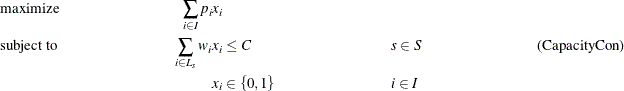
In this formulation, CapacityCon constraints ensure that the running tasks do not exceed the resource capacity. To illustrate,
consider the following five-task example with data: ![]() ,
, ![]() ,
, ![]() ,
, ![]() , and
, and ![]() . The formulation leads to a constraint matrix that has a staircase structure that is determined by tasks coming on and offline:
. The formulation leads to a constraint matrix that has a staircase structure that is determined by tasks coming on and offline:
![\[ \begin{array}{rlllllllllll} \mbox{maximize} & 6 x_1 & + & 8 x_2 & + & 5 x_3 & + & 9 x_4 & + & 8 x_5 \\ \mbox{subject to} & 8 x_1 & & & & & & & & & \leq & 10 \\ & 8 x_1 & + & 5 x_2 & & & & & & & \leq & 10 \\ & & & 5 x_2 & + & 3 x_3 & & & & & \leq & 10 \\ & & & 5 x_2 & + & 3 x_3 & + & 4 x_4 & & & \leq & 10 \\ & & & & + & 3 x_3 & + & 4 x_4 & + & 3 x_5 & \leq & 10 \\ & \multicolumn{11}{l}{x_ i \in \{ 0,1\} \quad i \in I}\\ \end{array} \]](images/ormpug_decomp0084.png)
This formulation clearly has no decomposable structure. However, you can use a common modeling technique known as Lagrangian decomposition to bring the model into block-angular form. Lagrangian decomposition works by first partitioning the constraints into blocks. Then, each original variable is split into multiple copies of itself, one copy for each block in which the variable has a nonzero coefficient in the constraint matrix. Constraints are added to enforce the equality of each copy of the original variable. Then, the original constraints can be written in block-angular form by using the duplicate variables.
To apply Lagrangian decomposition to the resource allocation problem, define a set B of blocks and let ![]() define the set of start times for a given block b, such that
define the set of start times for a given block b, such that ![]() . Given this partition of start times, let
. Given this partition of start times, let ![]() define the set of blocks in which task
define the set of blocks in which task ![]() is scheduled to be running. Now, for each task
is scheduled to be running. Now, for each task ![]() , define duplicate variables
, define duplicate variables ![]() for each
for each ![]() . Let
. Let ![]() define the minimum block index for each class of variable that represents task i. The problem can now be modeled in block-angular form as follows:
define the minimum block index for each class of variable that represents task i. The problem can now be modeled in block-angular form as follows:
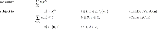
In this formulation, the LinkDupVarsCon constraints ensure that the duplicate variables are equal to the original variables. Now, the five-task example has been transformed from a staircase structure to a block-angular structure:
![\[ \begin{array}{r*{18}{r}} \mbox{maximize} & 6 x_1^1 & + & 8 x_2^1 & + & & & 5 x_3^2 & + & 9 x_4^2 & + & & & & & 8 x_5^3 \\ \mbox{subject to} & & & x_2^1 & - & x_2^2 & & & & & & & & & & & = & 0 \\ & & & & & & & x_3^2 & - & & & x_3^3 & & & & & = & 0 \\ & & & & & & & & & x_4^2 & & & - & x_4^3 & & & = & 0 \\ & 8 x_1^1 & & & & & & & & & & & & & & & \leq & 10 \\ & 8 x_1^1 & + & 5 x_2^1 & & & & & & & & & & & & & \leq & 10 \\ & & & & & 5 x_2^2 & + & 3 x_3^2 & & & & & & & & & \leq & 10 \\ & & & & & 5 x_2^2 & + & 3 x_3^2 & + & 4 x_4^2 & & & & & & & \leq & 10 \\ & & & & & & & & & & & 3 x_3^3 & + & 4 x_4^3 & + & 3 x_5^3 & \leq & 10 \\ & \multicolumn{11}{l}{x_ i^ b \in \{ 0,1\} \quad i \in I, \ b \in B_ i}\\ \end{array} \]](images/ormpug_decomp0092.png)
To show how to apply Lagrangian decomposition in PROC OPTMODEL, consider the following data set TaskData from Caprara, Furini, and Malaguti (2010) which consists of ![]() tasks:
tasks:
data TaskData;
   input profit weight start end;
   datalines;
100 74    1   12
 98 32    1    9
 73 27    1   22
 98 51    1   31
...
 23 40 2684 2689
 36 85 2685 2687
 65 44 2686 2689
 18 36 2687 2689
 88 57 2688 2689
;
The following PROC OPTMODEL statements read in the data and solve the original staircase formulation by calling the MILP solver directly:
%macro SetupData(task_data=, capacity=);
   set TASKS;
   num capacity=&capacity;
   num profit{TASKS}, weight{TASKS}, start{TASKS}, end{TASKS};

   read data &task_data into TASKS=[_n_] profit weight start end;
   /* the set of start times */

   set STARTS = setof{i in TASKS} start[i];
   /* the set of tasks i that are active at a given start time s */
   set TASKS_START{s in STARTS}
      = {i in TASKS: start[i] <= s < end[i]};
%mend SetupData;

%macro ResourceAllocation_Direct(task_data=, capacity=);
   proc optmodel;
      %SetupData(task_data=&task_data,capacity=&capacity);

      /* select task i to come online from period [start to end) */
      var x{TASKS} binary;

      /* maximize the total profit of running tasks */
      max TotalProfit = sum{i in TASKS} profit[i] * x[i];

      /* enforce that the shared resource capacity is not exceeded */
      con CapacityCon{s in STARTS}:
         sum{i in TASKS_START[s]} weight[i] * x[i] <= capacity;

      solve;
   quit;
%mend ResourceAllocation_Direct;

%ResourceAllocation_Direct(task_data=TaskData, capacity=100);
The problem summary and solution summary are displayed in Output 15.7.1.
Output 15.7.1: Problem Summary and Solution Summary
| Problem Summary | |
|---|---|
| Objective Sense | Maximization |
| Objective Function | TotalProfit |
| Objective Type | Linear |
| Number of Variables | 2697 |
| Bounded Above | 0 |
| Bounded Below | 0 |
| Bounded Below and Above | 2697 |
| Free | 0 |
| Fixed | 0 |
| Binary | 2697 |
| Integer | 0 |
| Number of Constraints | 2688 |
| Linear LE (<=) | 2688 |
| Linear EQ (=) | 0 |
| Linear GE (>=) | 0 |
| Linear Range | 0 |
| Constraint Coefficients | 26880 |
| Solution Summary | |
|---|---|
| Solver | MILP |
| Algorithm | Branch and Cut |
| Objective Function | TotalProfit |
| Solution Status | Optimal within Relative Gap |
| Objective Value | 62519.000416 |
| Relative Gap | 0.0000801027 |
| Absolute Gap | 5.0083389432 |
| Primal Infeasibility | 1.421085E-14 |
| Bound Infeasibility | 5.6710247E-7 |
| Integer Infeasibility | 7.2750423E-6 |
| Best Bound | 62524.008755 |
| Nodes | 849 |
| Iterations | 34532 |
| Presolve Time | 0.05 |
| Solution Time | 14.02 |
The iteration log, which contains the problem statistics, the progress of the solution, and the optimal objective value, is shown in Output 15.7.2.
Output 15.7.2: Log
| NOTE: There were 2697 observations read from the data set WORK.TASKDATA. |
| NOTE: Problem generation will use 4 threads. |
| NOTE: The problem has 2697 variables (0 free, 0 fixed). |
| NOTE: The problem has 2697 binary and 0 integer variables. |
| NOTE: The problem has 2688 linear constraints (2688 LE, 0 EQ, 0 GE, 0 range). |
| NOTE: The problem has 26880 linear constraint coefficients. |
| NOTE: The problem has 0 nonlinear constraints (0 LE, 0 EQ, 0 GE, 0 range). |
| NOTE: The OPTMODEL presolver is disabled for linear problems. |
| NOTE: The MILP presolver value AUTOMATIC is applied. |
| NOTE: The MILP presolver removed 0 variables and 0 constraints. |
| NOTE: The MILP presolver removed 0 constraint coefficients. |
| NOTE: The MILP presolver modified 0 constraint coefficients. |
| NOTE: The presolved problem has 2697 variables, 2688 constraints, and 26880 constraint |
| coefficients. |
| NOTE: The MILP solver is called. |
| Node Active Sols BestInteger BestBound Gap Time |
| 0 1 3 54182.0000000 145710 62.82% 0 |
| 0 1 3 54182.0000000 73230.2096818 26.01% 0 |
| 0 1 6 60619.0000000 68709.3995483 11.77% 0 |
| 0 1 7 61318.0000000 66335.8247833 7.56% 1 |
| 0 1 7 61318.0000000 64887.3843006 5.50% 2 |
| 0 1 7 61318.0000000 64027.1770833 4.23% 3 |
| 0 1 7 61318.0000000 63508.8490549 3.45% 3 |
| 0 1 7 61318.0000000 63201.3644716 2.98% 4 |
| 0 1 7 61318.0000000 63008.6642092 2.68% 4 |
| 0 1 7 61318.0000000 62915.6674025 2.54% 4 |
| 0 1 7 61318.0000000 62862.9976970 2.46% 4 |
| 0 1 7 61318.0000000 62835.8136672 2.42% 4 |
| 0 1 7 61318.0000000 62817.9245085 2.39% 4 |
| 0 1 7 61318.0000000 62801.4613187 2.36% 4 |
| 0 1 7 61318.0000000 62791.6244128 2.35% 4 |
| 0 1 7 61318.0000000 62787.2794961 2.34% 4 |
| 0 1 8 61432.0000000 62787.2794961 2.16% 4 |
| 0 1 8 61432.0000000 62787.2794961 2.16% 5 |
| NOTE: The MILP solver added 1255 cuts with 8485 cut coefficients at the root. |
| 100 97 8 61432.0000000 62754.5429591 2.11% 6 |
| 200 192 8 61432.0000000 62734.0925899 2.08% 8 |
| 300 287 8 61432.0000000 62690.7887512 2.01% 9 |
| 400 382 8 61432.0000000 62628.0076901 1.91% 10 |
| 500 478 8 61432.0000000 62614.7974543 1.89% 11 |
| 600 573 8 61432.0000000 62602.1443564 1.87% 12 |
| 700 668 8 61432.0000000 62585.9237739 1.84% 13 |
| 787 24 9 62503.0003956 62524.0686924 0.03% 13 |
| 800 36 9 62503.0003956 62524.0390976 0.03% 13 |
| 815 26 11 62514.0003173 62524.0390976 0.02% 13 |
| 848 4 13 62519.0004163 62524.0087553 0.01% 14 |
| NOTE: Optimal within relative gap. |
| NOTE: Objective = 62519.000416. |
To transform this data into block-angular form, first sort the task data to help reduce the number of duplicate variables needed in the reformulation as follows:
proc sort data=TaskData;
   by start end;
run;
Then, create the partition of constraints into blocks of size block_size as follows:
%macro ResourceAllocation_Decomp(task_data=, capacity=, block_size=);
   proc optmodel;
      %SetupData(task_data=&task_data,capacity=&capacity);
      /* partition into blocks of size blocks_size */
      num block_size = &block_size;
      num num_blocks = ceil( card(TASKS) / block_size );
      set BLOCKS     = 1..num_blocks;

      /* the set of starts s for which task i is active */
      set STARTS_TASK{i in TASKS} = {s in STARTS: start[i] <= s < end[i]};

      /* partition the start times into blocks of size block_size */
      set STARTS_BLOCK{BLOCKS} init {};
      num block_id    init 1;
      num block_count init 0;
      for{s in STARTS} do;
         STARTS_BLOCK[block_id] = STARTS_BLOCK[block_id] union {s};
         block_count = block_count + 1;
         if(mod(block_count, block_size) = 0) then
             block_id = block_id + 1;
      end;
Then, the following PROC OPTMODEL statements define the block-angular formulation and solve the problem by using the decomposition
algorithm, the PRESOLVER=BASIC option, and block_size=40. Because this reformulation is equivalent to the original staircase formulation, disabling some of the advanced presolver
techniques ensures that the model maintains block-angularity.
      /* blocks in which task i is online */
      set BLOCKS_TASK{i in TASKS} =
         {b in BLOCKS: card(STARTS_BLOCK[b] inter STARTS_TASK[i]) > 0};

      /* minimum block id in which task i is online */
      num min_block{i in TASKS} = min{b in BLOCKS_TASK[i]} b;

      /* select task i to come online from period [start to end)
         in each block */
      var x{i in TASKS, b in BLOCKS_TASK[i]} binary;

      /* maximize the total profit of running tasks */
      max TotalProfit = sum{i in TASKS} profit[i] * x[i,min_block[i]];

      /* enforce that task selection is consistent across blocks */
      con LinkDupVarsCon{i in TASKS, b in BLOCKS_TASK[i] diff {min_block[i]}}:
         x[i,b] = x[i,min_block[i]];

      /* enforce that the shared resource capacity is not exceeded */
      con CapacityCon{b in BLOCKS, s in STARTS_BLOCK[b]}:
         sum{i in TASKS_START[s]} weight[i] * x[i,b] <= capacity;

      /* define blocks for decomposition algorithm */
      for{b in BLOCKS, s in STARTS_BLOCK[b]} CapacityCon[b,s].block = b;

      solve with milp / presolver=basic decomp;
   quit;
%mend ResourceAllocation_Decomp;

%ResourceAllocation_Decomp(task_data=TaskData, capacity=100, block_size=40);
The problem summary and solution summary are displayed in Output 15.7.3. Compared to the original formulation, the number of variables and constraints is increased by the number of duplicate variables.
Output 15.7.3: Problem Summary and Solution Summary
| Problem Summary | |
|---|---|
| Objective Sense | Maximization |
| Objective Function | TotalProfit |
| Objective Type | Linear |
| Number of Variables | 3300 |
| Bounded Above | 0 |
| Bounded Below | 0 |
| Bounded Below and Above | 3300 |
| Free | 0 |
| Fixed | 0 |
| Binary | 3300 |
| Integer | 0 |
| Number of Constraints | 3291 |
| Linear LE (<=) | 2688 |
| Linear EQ (=) | 603 |
| Linear GE (>=) | 0 |
| Linear Range | 0 |
| Constraint Coefficients | 28086 |
| Solution Summary | |
|---|---|
| Solver | MILP |
| Algorithm | Decomposition |
| Objective Function | TotalProfit |
| Solution Status | Optimal within Relative Gap |
| Objective Value | 62524 |
| Relative Gap | 0.0000693019 |
| Absolute Gap | 4.3333333333 |
| Primal Infeasibility | 1.421085E-14 |
| Bound Infeasibility | 6.661338E-16 |
| Integer Infeasibility | 2.997602E-15 |
| Best Bound | 62528.333333 |
| Nodes | 14 |
| Iterations | 92 |
| Presolve Time | 0.07 |
| Solution Time | 15.97 |
The iteration log, which contains the problem statistics, the progress of the solution, and the optimal objective value, is shown in Output 15.7.4.
Output 15.7.4: Log
| NOTE: There were 2697 observations read from the data set WORK.TASKDATA. |
| NOTE: Problem generation will use 4 threads. |
| NOTE: The problem has 3300 variables (0 free, 0 fixed). |
| NOTE: The problem has 3300 binary and 0 integer variables. |
| NOTE: The problem has 3291 linear constraints (2688 LE, 603 EQ, 0 GE, 0 range). |
| NOTE: The problem has 28086 linear constraint coefficients. |
| NOTE: The problem has 0 nonlinear constraints (0 LE, 0 EQ, 0 GE, 0 range). |
| NOTE: The MILP presolver value BASIC is applied. |
| NOTE: The MILP presolver removed 0 variables and 0 constraints. |
| NOTE: The MILP presolver removed 0 constraint coefficients. |
| NOTE: The MILP presolver modified 0 constraint coefficients. |
| NOTE: The presolved problem has 3300 variables, 3291 constraints, and 28086 constraint |
| coefficients. |
| NOTE: The MILP solver is called. |
| NOTE: The Decomposition algorithm is used. |
| NOTE: The Decomposition algorithm is executing in single-machine mode. |
| NOTE: The DECOMP method value USER is applied. |
| NOTE: The problem has a decomposable structure with 68 blocks. The largest block covers 1.22% |
| of the constraints in the problem. |
| NOTE: The decomposition subproblems cover 3300 (100.00%) variables and 2688 (81.68%) |
| constraints. |
| NOTE: The deterministic parallel mode is enabled. |
| NOTE: The Decomposition algorithm is using up to 4 threads. |
| Iter Best Master Best LP IP CPU Real |
| Bound Objective Integer Gap Gap Time Time |
| NOTE: Starting phase 1. |
| 1 0.0000 0.0000 . 0.00% . 0 0 |
| NOTE: Starting phase 2. |
| 4 65890.0022 54643.0000 54643.0000 17.07% 17.07% 1 0 |
| 6 65890.0022 55803.0000 55803.0000 15.31% 15.31% 1 0 |
| 8 65890.0022 57033.0000 57033.0000 13.44% 13.44% 2 1 |
| 12 65890.0022 58656.3333 58649.0000 10.98% 10.99% 3 1 |
| 15 65890.0022 59958.3333 59951.0000 9.00% 9.01% 4 1 |
| 18 65890.0022 61274.0000 61274.0000 7.01% 7.01% 5 2 |
| 21 65890.0022 61450.0000 61402.0000 6.74% 6.81% 6 2 |
| 23 64827.4672 61755.0000 61707.0000 4.74% 4.81% 7 3 |
| 26 64188.2500 62160.0000 62160.0000 3.16% 3.16% 8 3 |
| 28 63540.6667 62228.0000 62228.0000 2.07% 2.07% 8 3 |
| . 63540.6667 62288.3333 62280.0000 1.97% 1.98% 9 4 |
| 30 63179.0000 62288.3333 62280.0000 1.41% 1.42% 9 4 |
| 31 63054.8333 62312.3333 62280.0000 1.18% 1.23% 10 4 |
| 32 62952.1728 62390.0833 62280.0000 0.89% 1.07% 11 4 |
| 33 62884.3374 62395.5833 62280.0000 0.78% 0.96% 11 5 |
| 37 62671.3333 62505.3333 62472.0000 0.26% 0.32% 12 5 |
| 38 62569.3333 62521.3333 62472.0000 0.08% 0.16% 13 5 |
| 39 62553.3333 62521.3333 62472.0000 0.05% 0.13% 13 6 |
| . 62553.3333 62527.3333 62472.0000 0.04% 0.13% 13 6 |
| 40 62553.3333 62527.3333 62472.0000 0.04% 0.13% 13 6 |
| 41 62534.3333 62527.3333 62472.0000 0.01% 0.10% 14 6 |
| 42 62528.3333 62527.3333 62472.0000 0.00% 0.09% 14 6 |
| NOTE: The Decomposition algorithm stopped on the continuous RELOBJGAP= option. |
| NOTE: Starting branch and bound. |
| Node Active Sols Best Best Gap CPU Real |
| Integer Bound Time Time |
| 0 1 26 62472.0000 62528.3333 0.09% 14 6 |
| 3 5 28 62509.0000 62528.3333 0.03% 22 10 |
| 5 5 30 62515.0000 62528.3333 0.02% 26 11 |
| 8 4 31 62522.0000 62528.3333 0.01% 32 13 |
| 10 2 31 62522.0000 62528.3333 0.01% 36 15 |
| 13 1 32 62524.0000 62528.3333 0.01% 37 15 |
| NOTE: The Decomposition algorithm used 4 threads. |
| NOTE: The Decomposition algorithm time is 15.77 seconds. |
| NOTE: Optimal within relative gap. |
| NOTE: Objective = 62524. |
The decomposition algorithm solves the problem in fewer nodes due to the stronger bound obtained by the reformulation. However,
it takes longer than the direct method to find a good feasible solution. The fact that the direct method seems to quickly
find good feasible solutions but has weaker bounds motivates the use of a hybrid algorithm. In the macro %ResourceAllocation_Decomp, replace the statement,
solve with milp / presolver=basic decomp;
with the following statements:
      solve with milp / relobjgap=0.1;
      solve with milp / presolver=basic primalin decomp;
These statements use the direct method with RELOBJGAP=0.1 to find a good starting solution and then use that result to seed the initial columns of the decomposition algorithm.
The solution summaries are displayed in Output 15.7.5.
Output 15.7.5: Solution Summaries
| Solution Summary | |
|---|---|
| Solver | MILP |
| Algorithm | Branch and Cut |
| Objective Function | TotalProfit |
| Solution Status | Optimal within Relative Gap |
| Objective Value | 61318 |
| Relative Gap | 0.0756427586 |
| Absolute Gap | 5017.8247833 |
| Primal Infeasibility | 0 |
| Bound Infeasibility | 2.220446E-16 |
| Integer Infeasibility | 2.220446E-16 |
| Best Bound | 66335.824783 |
| Nodes | 1 |
| Iterations | 3092 |
| Presolve Time | 0.06 |
| Solution Time | 1.73 |
| Solution Summary | |
|---|---|
| Solver | MILP |
| Algorithm | Decomposition |
| Objective Function | TotalProfit |
| Solution Status | Optimal within Relative Gap |
| Objective Value | 62524 |
| Relative Gap | 0.0000959539 |
| Absolute Gap | 6 |
| Primal Infeasibility | 2.220446E-16 |
| Bound Infeasibility | 6.661338E-16 |
| Integer Infeasibility | 6.661338E-16 |
| Best Bound | 62530 |
| Nodes | 3 |
| Iterations | 42 |
| Presolve Time | 0.07 |
| Solution Time | 7.66 |
The iteration log, which contains the problem statistics, the progress of the solution, and the optimal objective value, is shown in Output 15.7.6.
Output 15.7.6: Log
| NOTE: There were 2697 observations read from the data set WORK.TASKDATA. |
| NOTE: Problem generation will use 4 threads. |
| NOTE: The problem has 3300 variables (0 free, 0 fixed). |
| NOTE: The problem has 3300 binary and 0 integer variables. |
| NOTE: The problem has 3291 linear constraints (2688 LE, 603 EQ, 0 GE, 0 range). |
| NOTE: The problem has 28086 linear constraint coefficients. |
| NOTE: The problem has 0 nonlinear constraints (0 LE, 0 EQ, 0 GE, 0 range). |
| NOTE: The MILP presolver value AUTOMATIC is applied. |
| NOTE: The MILP presolver removed 603 variables and 603 constraints. |
| NOTE: The MILP presolver removed 1206 constraint coefficients. |
| NOTE: The MILP presolver modified 0 constraint coefficients. |
| NOTE: The presolved problem has 2697 variables, 2688 constraints, and 26880 constraint |
| coefficients. |
| NOTE: The MILP solver is called. |
| Node Active Sols BestInteger BestBound Gap Time |
| 0 1 3 54609.0000000 145710 62.52% 0 |
| 0 1 3 54609.0000000 73230.2096818 25.43% 0 |
| 0 1 6 60619.0000000 68709.3995483 11.77% 0 |
| 0 1 7 61318.0000000 66335.8247833 7.56% 1 |
| NOTE: The MILP solver added 734 cuts with 3910 cut coefficients at the root. |
| NOTE: Optimal within relative gap. |
| NOTE: Objective = 61318. |
| NOTE: The MILP presolver value BASIC is applied. |
| NOTE: The MILP presolver removed 0 variables and 0 constraints. |
| NOTE: The MILP presolver removed 0 constraint coefficients. |
| NOTE: The MILP presolver modified 0 constraint coefficients. |
| NOTE: The presolved problem has 3300 variables, 3291 constraints, and 28086 constraint |
| coefficients. |
| NOTE: The MILP solver is called. |
| NOTE: The Decomposition algorithm is used. |
| NOTE: The Decomposition algorithm is executing in single-machine mode. |
| NOTE: The DECOMP method value USER is applied. |
| NOTE: The problem has a decomposable structure with 68 blocks. The largest block covers 1.22% |
| of the constraints in the problem. |
| NOTE: The decomposition subproblems cover 3300 (100.00%) variables and 2688 (81.68%) |
| constraints. |
| NOTE: The deterministic parallel mode is enabled. |
| NOTE: The Decomposition algorithm is using up to 4 threads. |
| Iter Best Master Best LP IP CPU Real |
| Bound Objective Integer Gap Gap Time Time |
| NOTE: Starting phase 1. |
| 1 0.0000 0.0000 . 0.00% . 0 0 |
| NOTE: Starting phase 2. |
| 2 65890.0003 61360.0000 61360.0000 6.88% 6.88% 1 0 |
| 5 65890.0003 61379.0000 61379.0000 6.85% 6.85% 1 0 |
| 6 65890.0003 61406.0000 61406.0000 6.81% 6.81% 2 0 |
| 8 65890.0003 61571.0000 61571.0000 6.55% 6.55% 3 1 |
| . 65890.0003 61733.0000 61733.0000 6.31% 6.31% 3 1 |
| 10 65439.0015 61733.0000 61733.0000 5.66% 5.66% 4 1 |
| 12 64743.5001 61827.0000 61827.0000 4.50% 4.50% 4 1 |
| 13 64743.5001 61934.0000 61934.0000 4.34% 4.34% 5 2 |
| 15 64743.5001 62139.0000 62094.0000 4.02% 4.09% 6 2 |
| 17 63631.2500 62284.0000 62224.0000 2.12% 2.21% 7 2 |
| 18 62964.7500 62299.0000 62239.0000 1.06% 1.15% 7 3 |
| . 62964.7500 62443.4667 62351.0000 0.83% 0.97% 8 3 |
| 21 62920.9333 62443.4667 62351.0000 0.76% 0.91% 9 3 |
| 22 62773.5013 62472.8333 62351.0000 0.48% 0.67% 9 4 |
| 25 62707.5000 62507.3333 62496.0000 0.32% 0.34% 10 4 |
| 27 62583.3335 62522.3333 62505.0000 0.10% 0.13% 10 4 |
| 28 62580.3339 62522.3333 62505.0000 0.09% 0.12% 11 5 |
| 29 62537.3333 62522.3333 62505.0000 0.02% 0.05% 11 5 |
| . 62537.3333 62528.3333 62524.0000 0.01% 0.02% 11 5 |
| 30 62537.3333 62528.3333 62524.0000 0.01% 0.02% 11 5 |
| 31 62536.3333 62528.3333 62524.0000 0.01% 0.02% 12 5 |
| 32 62532.8333 62528.3333 62524.0000 0.01% 0.01% 12 5 |
| NOTE: The Decomposition algorithm stopped on the continuous RELOBJGAP= option. |
| NOTE: Starting branch and bound. |
| Node Active Sols Best Best Gap CPU Real |
| Integer Bound Time Time |
| 0 1 21 62524.0000 62532.8333 0.01% 12 5 |
| 2 0 21 62524.0000 62530.0000 0.01% 17 7 |
| NOTE: The Decomposition algorithm used 4 threads. |
| NOTE: The Decomposition algorithm time is 7.46 seconds. |
| NOTE: Optimal within relative gap. |
| NOTE: Objective = 62524. |
By using this hybrid method, you can take advantage of the direct method, which finds a good feasible solution quickly, and the strong bounds provided by the decomposition algorithm.
Alternatively, you can use the built-in hybrid method in one call to the solver by using the HYBRID=ON option in the DECOMP
statement. This algorithm first processes the root node by using standard MILP techniques. It then proceeds with the decomposition
algorithm to complete processing. In the macro %ResourceAllocation_Decomp, replace the statement
solve with milp / presolver=basic decomp;
with the statement
solve with milp / presolver=basic decomp=(hybrid=on);
The solution summary is displayed in Output 15.7.7.
Output 15.7.7: Solution Summary
| Solution Summary | |
|---|---|
| Solver | MILP |
| Algorithm | Decomposition |
| Objective Function | TotalProfit |
| Solution Status | Optimal within Relative Gap |
| Objective Value | 62524 |
| Relative Gap | 0.0000693019 |
| Absolute Gap | 4.3333333333 |
| Primal Infeasibility | 4.263256E-14 |
| Bound Infeasibility | 8.881784E-16 |
| Integer Infeasibility | 8.881784E-16 |
| Best Bound | 62528.333333 |
| Nodes | 4 |
| Iterations | 41 |
| Presolve Time | 0.08 |
| Solution Time | 14.71 |
The iteration log, which contains the problem statistics, the progress of the solution, and the optimal objective value, is shown in Output 15.7.8.
Output 15.7.8: Log
| NOTE: There were 2697 observations read from the data set WORK.TASKDATA. |
| NOTE: Problem generation will use 4 threads. |
| NOTE: The problem has 3300 variables (0 free, 0 fixed). |
| NOTE: The problem has 3300 binary and 0 integer variables. |
| NOTE: The problem has 3291 linear constraints (2688 LE, 603 EQ, 0 GE, 0 range). |
| NOTE: The problem has 28086 linear constraint coefficients. |
| NOTE: The problem has 0 nonlinear constraints (0 LE, 0 EQ, 0 GE, 0 range). |
| NOTE: The MILP presolver value BASIC is applied. |
| NOTE: The MILP presolver removed 0 variables and 0 constraints. |
| NOTE: The MILP presolver removed 0 constraint coefficients. |
| NOTE: The MILP presolver modified 0 constraint coefficients. |
| NOTE: The presolved problem has 3300 variables, 3291 constraints, and 28086 constraint |
| coefficients. |
| NOTE: The Decomposition algorithm is using the direct MILP solver for the root node. |
| NOTE: The MILP solver is called. |
| Node Active Sols BestInteger BestBound Gap Time |
| 0 1 3 52549.0000000 73230.2096818 28.24% 0 |
| 0 1 6 60129.0000000 68724.4564404 12.51% 1 |
| 0 1 8 60352.0000000 66375.4142650 9.07% 2 |
| 0 1 8 60352.0000000 64959.3967107 7.09% 2 |
| 0 1 8 60352.0000000 64022.2814465 5.73% 3 |
| 0 1 8 60352.0000000 63561.9969629 5.05% 4 |
| 0 1 8 60352.0000000 63192.8473290 4.50% 5 |
| 0 1 8 60352.0000000 62995.6489462 4.20% 5 |
| 0 1 8 60352.0000000 62927.0282767 4.09% 5 |
| 0 1 8 60352.0000000 62877.9947740 4.02% 5 |
| 0 1 8 60352.0000000 62840.8625639 3.96% 5 |
| 0 1 8 60352.0000000 62821.1059108 3.93% 5 |
| 0 1 8 60352.0000000 62809.7299610 3.91% 6 |
| 0 1 8 60352.0000000 62795.8029927 3.89% 6 |
| 0 1 8 60352.0000000 62783.6627781 3.87% 6 |
| 0 1 9 60912.0000000 62783.6627781 2.98% 6 |
| NOTE: The MILP solver added 1286 cuts with 8726 cut coefficients at the root. |
| NOTE: The Decomposition algorithm is used. |
| NOTE: The Decomposition algorithm is executing in single-machine mode. |
| NOTE: The DECOMP method value USER is applied. |
| NOTE: The problem has a decomposable structure with 68 blocks. The largest block covers 1.49% |
| of the constraints in the problem. |
| NOTE: The decomposition subproblems cover 3300 (100.00%) variables and 3930 (85.86%) |
| constraints. |
| NOTE: The deterministic parallel mode is enabled. |
| NOTE: The Decomposition algorithm is using up to 4 threads. |
| Iter Best Master Best LP IP CPU Real |
| Bound Objective Integer Gap Gap Time Time |
| NOTE: Starting phase 1. |
| 1 0.0000 0.0000 . 0.00% . 0 0 |
| NOTE: Starting phase 2. |
| 3 62783.6628 61679.0000 61679.0000 1.76% 1.76% 0 0 |
| 6 62783.6628 61776.0000 61776.0000 1.60% 1.60% 1 0 |
| 8 62783.6628 61860.5000 61844.0000 1.47% 1.50% 2 0 |
| . 62783.6628 61892.5000 61876.0000 1.42% 1.45% 2 1 |
| 10 62783.6628 61892.5000 61876.0000 1.42% 1.45% 2 1 |
| 13 62783.6628 62068.5000 62052.0000 1.14% 1.17% 3 1 |
| 17 62783.6628 62290.3333 62286.0000 0.79% 0.79% 5 2 |
| 19 62783.6628 62366.3333 62347.0000 0.66% 0.70% 6 3 |
| 22 62783.6628 62407.3333 62390.0000 0.60% 0.63% 7 3 |
| 24 62704.3336 62472.3333 62390.0000 0.37% 0.50% 9 4 |
| 26 62628.5000 62515.3333 62498.0000 0.18% 0.21% 9 4 |
| 27 62573.3340 62515.3333 62498.0000 0.09% 0.12% 10 4 |
| 28 62564.3333 62520.3333 62498.0000 0.07% 0.11% 10 5 |
| 29 62543.3333 62521.3333 62499.0000 0.04% 0.07% 11 5 |
| . 62543.3333 62521.3333 62512.0000 0.04% 0.05% 11 5 |
| 30 62528.3333 62521.3333 62512.0000 0.01% 0.03% 11 5 |
| NOTE: The Decomposition algorithm stopped on the continuous RELOBJGAP= option. |
| . 62528.3333 62523.3333 62514.0000 0.01% 0.02% 11 6 |
| NOTE: Starting branch and bound. |
| Node Active Sols Best Best Gap CPU Real |
| Integer Bound Time Time |
| 0 1 27 62514.0000 62528.3333 0.02% 11 6 |
| 3 1 28 62524.0000 62528.3333 0.01% 16 8 |
| NOTE: The Decomposition algorithm used 4 threads. |
| NOTE: The Decomposition algorithm time is 8.49 seconds. |
| NOTE: Optimal within relative gap. |
| NOTE: Objective = 62524. |
The reformulation of this resource allocation problem provides a nice example of the potential tradeoffs in modeling a problem
for use with the decomposition algorithm. As seen in Example 15.2, the strength of the bound is an important factor in the overall performance of the algorithm, but it is not always correlated
to the magnitude of the subproblem coverage. In this example, the block size determines the number of blocks. Moreover, it
determines the number of linking variables that are needed in the reformulation. At one extreme, if the block size is set
to be ![]() , then the number of blocks is 1, and the number of copies of original variables is 0. Using one block would be equivalent
to the original staircase formulation and would not yield a model conducive to decomposition. As the number of blocks is increased,
the number of linking variables increases (the size of the master problem), the strength of the decomposition bound decreases,
and the difficulty of solving the subproblems decreases. In addition, as the number of blocks and their relative difficulty
change, the efficient utilization of your machine’s parallel architecture can be affected.
, then the number of blocks is 1, and the number of copies of original variables is 0. Using one block would be equivalent
to the original staircase formulation and would not yield a model conducive to decomposition. As the number of blocks is increased,
the number of linking variables increases (the size of the master problem), the strength of the decomposition bound decreases,
and the difficulty of solving the subproblems decreases. In addition, as the number of blocks and their relative difficulty
change, the efficient utilization of your machine’s parallel architecture can be affected.
The previous section used a block size of 40. The following statement calls the decomposition algorithm and uses a block size of 130:
%ResourceAllocation_Decomp(task_data=TaskData, capacity=100, block_size=130);
The solution summary is displayed in Output 15.7.9.
Output 15.7.9: Solution Summary
| Solution Summary | |
|---|---|
| Solver | MILP |
| Algorithm | Decomposition |
| Objective Function | TotalProfit |
| Solution Status | Optimal within Relative Gap |
| Objective Value | 62524 |
| Relative Gap | 0.0000959539 |
| Absolute Gap | 6 |
| Primal Infeasibility | 1.110223E-15 |
| Bound Infeasibility | 4.440892E-16 |
| Integer Infeasibility | 1.887379E-15 |
| Best Bound | 62530 |
| Nodes | 1 |
| Iterations | 22 |
| Presolve Time | 0.06 |
| Solution Time | 6.62 |
The iteration log, which contains the problem statistics, the progress of the solution, and the optimal objective value, is shown in Output 15.7.10.
Output 15.7.10: Log
| NOTE: There were 2697 observations read from the data set WORK.TASKDATA. |
| NOTE: Problem generation will use 4 threads. |
| NOTE: The problem has 2877 variables (0 free, 0 fixed). |
| NOTE: The problem has 2877 binary and 0 integer variables. |
| NOTE: The problem has 2868 linear constraints (2688 LE, 180 EQ, 0 GE, 0 range). |
| NOTE: The problem has 27240 linear constraint coefficients. |
| NOTE: The problem has 0 nonlinear constraints (0 LE, 0 EQ, 0 GE, 0 range). |
| NOTE: The MILP presolver value BASIC is applied. |
| NOTE: The MILP presolver removed 0 variables and 0 constraints. |
| NOTE: The MILP presolver removed 0 constraint coefficients. |
| NOTE: The MILP presolver modified 0 constraint coefficients. |
| NOTE: The presolved problem has 2877 variables, 2868 constraints, and 27240 constraint |
| coefficients. |
| NOTE: The MILP solver is called. |
| NOTE: The Decomposition algorithm is used. |
| NOTE: The Decomposition algorithm is executing in single-machine mode. |
| NOTE: The DECOMP method value USER is applied. |
| NOTE: The problem has a decomposable structure with 21 blocks. The largest block covers 4.53% |
| of the constraints in the problem. |
| NOTE: The decomposition subproblems cover 2877 (100.00%) variables and 2688 (93.72%) |
| constraints. |
| NOTE: The deterministic parallel mode is enabled. |
| NOTE: The Decomposition algorithm is using up to 4 threads. |
| Iter Best Master Best LP IP CPU Real |
| Bound Objective Integer Gap Gap Time Time |
| NOTE: Starting phase 1. |
| 1 0.0000 0.0000 . 0.00% . 1 0 |
| NOTE: Starting phase 2. |
| 4 63337.0040 58365.0000 58365.0000 7.85% 7.85% 3 1 |
| 6 63337.0040 59142.0000 59142.0000 6.62% 6.62% 5 1 |
| 9 63337.0040 61339.0000 61339.0000 3.15% 3.15% 6 2 |
| 11 63337.0040 61786.0000 61775.0000 2.45% 2.47% 8 2 |
| 13 63337.0040 62230.0000 62230.0000 1.75% 1.75% 10 3 |
| 15 62956.0002 62263.0000 62263.0000 1.10% 1.10% 13 4 |
| 17 62904.0000 62467.0000 62467.0000 0.69% 0.69% 14 5 |
| 18 62808.0008 62482.5000 62467.0000 0.52% 0.54% 16 5 |
| . 62808.0008 62524.0000 62524.0000 0.45% 0.45% 16 5 |
| 20 62726.6687 62524.0000 62524.0000 0.32% 0.32% 17 5 |
| 21 62600.5000 62524.0000 62524.0000 0.12% 0.12% 17 6 |
| 22 62530.0000 62524.0000 62524.0000 0.01% 0.01% 18 6 |
| NOTE: The Decomposition algorithm stopped on the integer RELOBJGAP= option. |
| Node Active Sols Best Best Gap CPU Real |
| Integer Bound Time Time |
| 0 0 17 62524.0000 62530.0000 0.01% 18 6 |
| NOTE: The Decomposition algorithm used 4 threads. |
| NOTE: The Decomposition algorithm time is 6.45 seconds. |
| NOTE: Optimal within relative gap. |
| NOTE: Objective = 62524. |
This version of the model provides a stronger bound and requires a smaller branch-and-bound search tree to find an optimal solution.