The Decomposition Algorithm
- Overview
-
Getting Started

-
SyntaxDecomposition Algorithm Options in the PROC OPTLP Statement or the SOLVE WITH LP Statement in PROC OPTMODELDecomposition Algorithm Options in the PROC OPTMILP Statement or the SOLVE WITH MILP Statement in PROC OPTMODELDECOMP StatementDECOMP_MASTER StatementDECOMP_MASTER_IP StatementDECOMP_SUBPROB Statement
-
Details
-
ExamplesMulticommodity Flow ProblemGeneralized Assignment ProblemBlock-Diagonal Structure and METHOD=CONCOMP in Single-Machine ModeBlock-Diagonal Structure and METHOD=CONCOMP in Distributed ModeBlock-Angular Structure and METHOD=AUTOBin Packing ProblemResource Allocation ProblemVehicle Routing ProblemATM Cash Management in Single-Machine ModeATM Cash Management in Distributed ModeKidney Donor Exchange
- References
The generalized assignment problem (GAP) is that of finding a maximum profit assignment from n tasks to m machines such that each task is assigned to precisely one machine subject to capacity restrictions on the machines. With
each possible assignment, associate a binary variable ![]() , which, if set to 1, indicates that machine i is assigned to task j. For ease of notation, define two index sets
, which, if set to 1, indicates that machine i is assigned to task j. For ease of notation, define two index sets ![]() and
and ![]() . A GAP can be formulated as a MILP as follows:
. A GAP can be formulated as a MILP as follows:
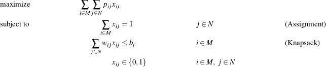
In this formulation, Assignment constraints ensure that each task is assigned to exactly one machine. Knapsack constraints ensure that for each machine, the capacity restrictions are met.
Consider the following example taken from Koch et al. (2011) with ![]() tasks to be assigned to
tasks to be assigned to ![]() machines. The data set
machines. The data set profit_data provides the profit for assigning a particular task to a particular machine:
%let NumTasks    = 24;
%let NumMachines = 8;

data profit_data;
   input p1-p&NumTasks;
   datalines;
25 23 20 16 19 22 20 16 15 22 15 21 20 23 20 22 19 25 25 24 21 17 23 17
16 19 22 22 19 23 17 24 15 24 18 19 20 24 25 25 19 24 18 21 16 25 15 20
20 18 23 23 23 17 19 16 24 24 17 23 19 22 23 25 23 18 19 24 20 17 23 23
16 16 15 23 15 15 25 22 17 20 19 16 17 17 20 17 17 18 16 18 15 25 22 17
17 23 21 20 24 22 25 17 22 20 16 22 21 23 24 15 22 25 18 19 19 17 22 23
24 21 23 17 21 19 19 17 18 24 15 15 17 18 15 24 19 21 23 24 17 20 16 21
18 21 22 23 22 15 18 15 21 22 15 23 21 25 25 23 20 16 25 17 15 15 18 16
19 24 18 17 21 18 24 25 18 23 21 15 24 23 18 18 23 23 16 20 20 19 25 21
;
The data set weight_data provides the amount of resources used by a particular task when assigned to a particular machine:
data weight_data;
   input w1-w&NumTasks;
   datalines;
 8 18 22  5 11 11 22 11 17 22 11 20 13 13  7 22 15 22 24  8  8 24 18  8
24 14 11 15 24  8 10 15 19 25  6 13 10 25 19 24 13 12  5 18 10 24  8  5
22 22 21 22 13 16 21  5 25 13 12  9 24  6 22 24 11 21 11 14 12 10 20  6
13  8 19 12 19 18 10 21  5  9 11  9 22  8 12 13  9 25 19 24 22  6 19 14
25 16 13  5 11  8  7  8 25 20 24 20 11  6 10 10  6 22 10 10 13 21  5 19
19 19  5 11 22 24 18 11  6 13 24 24 22  6 22  5 14  6 16 11  6  8 18 10
24 10  9 10  6 15  7 13 20  8  7  9 24  9 21  9 11 19 10  5 23 20  5 21
 6  9  9  5 12 10 16 15 19 18 20 18 16 21 11 12 22 16 21 25  7 14 16 10
;
Finally, the data set capacity_data provides the resource capacity for each machine:
data capacity_data;
   input b @@;
   datalines;
36 35 38 34 32 34 31 34
;
The following PROC OPTMODEL statements read in the data and define the necessary sets and parameters:
proc optmodel;
   /* declare index sets */
   set TASKS    = 1..&NumTasks;
   set MACHINES = 1..&NumMachines;

   /* declare parameters */
   num profit   {MACHINES, TASKS};
   num weight   {MACHINES, TASKS};
   num capacity {MACHINES};

   /* read data sets to populate data */
   read data profit_data   into [i=_n_] {j in TASKS} <profit[i,j]=col('p'||j)>;
   read data weight_data   into [i=_n_] {j in TASKS} <weight[i,j]=col('w'||j)>;
   read data capacity_data into [_n_] capacity=b;
The following statements declare the optimization model:
   /* declare decision variables */
   var Assign {MACHINES, TASKS} binary;

   /* declare objective */
   max TotalProfit =
      sum {i in MACHINES, j in TASKS} profit[i,j] * Assign[i,j];

   /* declare constraints */
   con Assignment {j in TASKS}:
      sum {i in MACHINES} Assign[i,j] = 1;

   con Knapsack {i in MACHINES}:
      sum {j in TASKS} weight[i,j] * Assign[i,j] <= capacity[i];
The following statements use two different decompositions to solve the problem. The first decomposition defines each Assignment constraint as a block and uses the pure network simplex solver for the subproblem. The second decomposition defines each Knapsack constraint as a block and uses the MILP solver for the subproblem.
   /* each Assignment constraint defines a block */
   for{j in TASKS}
      Assignment[j].block = j;

   solve with milp / logfreq=1000
      decomp        =()
      decomp_subprob=(algorithm=nspure);

   /* each Knapsack constraint defines a block */
   for{j in TASKS}
      Assignment[j].block = .;
   for{i in MACHINES}
      Knapsack[i].block = i;

   solve with milp / decomp;
quit;
The solution summaries are displayed in Output 15.2.1.
Output 15.2.1: Solution Summaries
| Solution Summary | |
|---|---|
| Solver | MILP |
| Algorithm | Decomposition |
| Objective Function | TotalProfit |
| Solution Status | Optimal within Relative Gap |
| Objective Value | 563 |
| Relative Gap | 0.0000925018 |
| Absolute Gap | 0.0520833333 |
| Primal Infeasibility | 6.661338E-16 |
| Bound Infeasibility | 2.220446E-16 |
| Integer Infeasibility | 6.661338E-16 |
| Best Bound | 563.05208333 |
| Nodes | 1763 |
| Iterations | 1802 |
| Presolve Time | 0.00 |
| Solution Time | 4.46 |
| Solution Summary | |
|---|---|
| Solver | MILP |
| Algorithm | Decomposition |
| Objective Function | TotalProfit |
| Solution Status | Optimal |
| Objective Value | 563 |
| Relative Gap | 0 |
| Absolute Gap | 0 |
| Primal Infeasibility | 0 |
| Bound Infeasibility | 0 |
| Integer Infeasibility | 0 |
| Best Bound | 563 |
| Nodes | 3 |
| Iterations | 33 |
| Presolve Time | 0.01 |
| Solution Time | 0.24 |
The iteration log for both decompositions is shown in Output 15.2.2. This example is interesting because it shows the tradeoff between the strength of the relaxation and the difficulty of its resolution. In the first decomposition, the subproblems are totally unimodular and can be solved trivially. Consequently, each iteration of the decomposition algorithm is very fast. However, the bound obtained is as weak as the bound found in direct methods (the LP bound). The weaker bound leads to the need to enumerate more nodes overall. Alternatively, in the second decomposition, the subproblem is the knapsack problem, which is solved using MILP. In this case, the bound is much tighter and the problem solves in very few nodes. The tradeoff, of course, is that each iteration takes longer because solving the knapsack problem is not trivial. Another interesting aspect of this problem is that the subproblem coverage in the second decomposition is much smaller than that of the first decomposition. However, when dealing with MILP, it is not always the size of the coverage that determines the overall effectiveness of a particular choice of decomposition.
Output 15.2.2: Log
| NOTE: There were 8 observations read from the data set WORK.PROFIT_DATA. |
| NOTE: There were 8 observations read from the data set WORK.WEIGHT_DATA. |
| NOTE: There were 8 observations read from the data set WORK.CAPACITY_DATA. |
| NOTE: Problem generation will use 4 threads. |
| NOTE: The problem has 192 variables (0 free, 0 fixed). |
| NOTE: The problem has 192 binary and 0 integer variables. |
| NOTE: The problem has 32 linear constraints (8 LE, 24 EQ, 0 GE, 0 range). |
| NOTE: The problem has 384 linear constraint coefficients. |
| NOTE: The problem has 0 nonlinear constraints (0 LE, 0 EQ, 0 GE, 0 range). |
| NOTE: The MILP presolver value AUTOMATIC is applied. |
| NOTE: The MILP presolver removed 0 variables and 0 constraints. |
| NOTE: The MILP presolver removed 0 constraint coefficients. |
| NOTE: The MILP presolver modified 0 constraint coefficients. |
| NOTE: The presolved problem has 192 variables, 32 constraints, and 384 constraint coefficients. |
| NOTE: The MILP solver is called. |
| NOTE: The Decomposition algorithm is used. |
| NOTE: The Decomposition algorithm is executing in single-machine mode. |
| NOTE: The DECOMP method value USER is applied. |
| NOTE: The subproblem solver chosen is an LP solver but at least one block has integer variables. |
| NOTE: The problem has a decomposable structure with 24 blocks. The largest block covers 3.13% |
| of the constraints in the problem. |
| NOTE: The decomposition subproblems cover 192 (100.00%) variables and 24 (75.00%) constraints. |
| NOTE: The deterministic parallel mode is enabled. |
| NOTE: The Decomposition algorithm is using up to 4 threads. |
| Iter Best Master Best LP IP CPU Real |
| Bound Objective Integer Gap Gap Time Time |
| NOTE: Starting phase 1. |
| 1 0.0000 8.9248 . 8.92e+00 . 0 0 |
| 4 0.0000 0.0000 . 0.00% . 0 0 |
| NOTE: Starting phase 2. |
| 5 574.0000 561.1587 . 2.24% . 0 0 |
| 6 568.8833 568.5610 . 0.06% . 0 0 |
| 8 568.6464 568.6464 560.0000 0.00% 1.52% 0 0 |
| NOTE: Starting branch and bound. |
| Node Active Sols Best Best Gap CPU Real |
| Integer Bound Time Time |
| 0 1 1 560.0000 568.6464 1.52% 0 0 |
| 5 7 2 563.0000 568.4782 0.96% 0 0 |
| 1000 432 2 563.0000 564.6212 0.29% 2 2 |
| 1762 0 2 563.0000 563.0521 0.01% 4 4 |
| NOTE: The Decomposition algorithm used 4 threads. |
| NOTE: The Decomposition algorithm time is 4.46 seconds. |
| NOTE: Optimal within relative gap. |
| NOTE: Objective = 563. |
| NOTE: The MILP presolver value AUTOMATIC is applied. |
| NOTE: The MILP presolver removed 0 variables and 0 constraints. |
| NOTE: The MILP presolver removed 0 constraint coefficients. |
| NOTE: The MILP presolver modified 0 constraint coefficients. |
| NOTE: The presolved problem has 192 variables, 32 constraints, and 384 constraint coefficients. |
| NOTE: The MILP solver is called. |
| NOTE: The Decomposition algorithm is used. |
| NOTE: The Decomposition algorithm is executing in single-machine mode. |
| NOTE: The DECOMP method value USER is applied. |
| NOTE: The problem has a decomposable structure with 8 blocks. The largest block covers 3.13% of |
| the constraints in the problem. |
| NOTE: The decomposition subproblems cover 192 (100.00%) variables and 8 (25.00%) constraints. |
| NOTE: The deterministic parallel mode is enabled. |
| NOTE: The Decomposition algorithm is using up to 4 threads. |
| Iter Best Master Best LP IP CPU Real |
| Bound Objective Integer Gap Gap Time Time |
| NOTE: Starting phase 1. |
| 1 0.0000 10.0000 . 1.00e+01 . 0 0 |
| 8 0.0000 0.0000 . 0.00% . 0 0 |
| NOTE: Starting phase 2. |
| 11 717.5556 540.0000 540.0000 24.74% 24.74% 0 0 |
| 13 670.3333 548.0000 548.0000 18.25% 18.25% 0 0 |
| 14 627.9557 548.0000 548.0000 12.73% 12.73% 0 0 |
| 16 592.2500 549.8750 548.0000 7.15% 7.47% 0 0 |
| 19 592.2500 558.0000 558.0000 5.78% 5.78% 0 0 |
| . 592.2500 558.0000 558.0000 5.78% 5.78% 0 0 |
| 20 577.6667 558.0000 558.0000 3.40% 3.40% 0 0 |
| 23 574.6667 560.6667 560.0000 2.44% 2.55% 0 0 |
| 24 574.6667 563.0000 563.0000 2.03% 2.03% 0 0 |
| 25 569.5000 563.5000 563.0000 1.05% 1.14% 0 0 |
| 26 566.1905 563.7143 563.0000 0.44% 0.56% 0 0 |
| 28 564.5000 564.0000 563.0000 0.09% 0.27% 0 0 |
| 29 564.0000 564.0000 563.0000 0.00% 0.18% 0 0 |
| NOTE: Starting branch and bound. |
| Node Active Sols Best Best Gap CPU Real |
| Integer Bound Time Time |
| 0 1 8 563.0000 564.0000 0.18% 0 0 |
| 4 0 8 563.0000 563.0000 0.00% 0 0 |
| NOTE: The Decomposition algorithm used 4 threads. |
| NOTE: The Decomposition algorithm time is 0.15 seconds. |
| NOTE: Optimal. |
| NOTE: Objective = 563. |