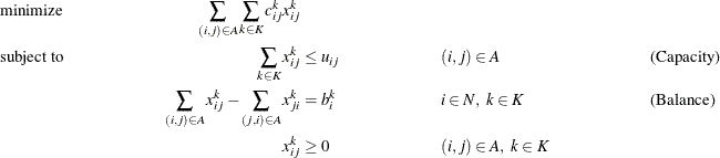
The Decomposition Algorithm
- Overview
-
Getting Started

-
SyntaxDecomposition Algorithm Options in the PROC OPTLP Statement or the SOLVE WITH LP Statement in PROC OPTMODELDecomposition Algorithm Options in the PROC OPTMILP Statement or the SOLVE WITH MILP Statement in PROC OPTMODELDECOMP StatementDECOMP_MASTER StatementDECOMP_MASTER_IP StatementDECOMP_SUBPROB Statement
-
Details
-
ExamplesMulticommodity Flow ProblemGeneralized Assignment ProblemBlock-Diagonal Structure and METHOD=CONCOMP in Single-Machine ModeBlock-Diagonal Structure and METHOD=CONCOMP in Distributed ModeBlock-Angular Structure and METHOD=AUTOBin Packing ProblemResource Allocation ProblemVehicle Routing ProblemATM Cash Management in Single-Machine ModeATM Cash Management in Distributed ModeKidney Donor Exchange
- References
This example demonstrates how to use the decomposition algorithm to find a minimum-cost multicommodity flow (MMCF) in a directed network. This type of problem was motivation for the development of the original Dantzig-Wolfe decomposition method (Dantzig and Wolfe, 1960).
Let ![]() be a directed graph, and let K be a set of commodities. For each link
be a directed graph, and let K be a set of commodities. For each link ![]() and each commodity k, associate a cost per unit of flow, designated by
and each commodity k, associate a cost per unit of flow, designated by ![]() . The demand (or supply) at each node
. The demand (or supply) at each node ![]() for commodity k is designated as
for commodity k is designated as ![]() , where
, where ![]() denotes a supply node and
denotes a supply node and ![]() denotes a demand node. Define decision variables
denotes a demand node. Define decision variables ![]() that denote the amount of commodity k sent from node i and node j. The amount of total flow, across all commodities, that can be sent across each link is bounded above by
that denote the amount of commodity k sent from node i and node j. The amount of total flow, across all commodities, that can be sent across each link is bounded above by ![]() .
.
The problem can be modeled as a linear programming problem as follows:
In this formulation, The Capacity constraints limit the total flow across all commodities on each arc. The Balance constraints ensure that the flow of commodities leaving each supply node and entering each demand node are balanced.
Consider the directed graph in Figure 15.5 which appears in Ahuja, Magnanti, and Orlin (1993).
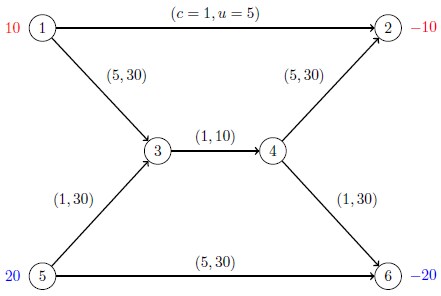
The goal in this example is to minimize the total cost of sending two commodities across the network while satisfying all supplies and demands and respecting arc capacities. If there were no arc capacities linking the two commodities, you could solve a separate minimum-cost network flow problem for each commodity one at a time.
The following data set arc_comm_data provides the cost ![]() of sending a unit of commodity k along arc
of sending a unit of commodity k along arc ![]() :
:
data arc_comm_data;
   input k i j cost;
   datalines;
1 1 2 1
1 1 3 5
1 5 3 1
1 5 6 5
1 3 4 1
1 4 2 5
1 4 6 1
2 1 2 1
2 1 3 5
2 5 3 1
2 5 6 5
2 3 4 1
2 4 2 5
2 4 6 1
;
Next, the data set arc_data provides the capacity ![]() for each arc:
for each arc:
data arc_data;
   input i j capacity;
   datalines;
1 2  5
1 3 30
5 3 30
5 6 30
3 4 10
4 2 30
4 6 30
;
data supply_data;
   input k i supply;
   datalines;
1 1  10
1 2 -10
2 5  20
2 6 -20
;
The following PROC OPTMODEL statements find the minimum-cost multicommodity flow:
proc optmodel;
   set <num,num,num> ARC_COMM;
   num cost {ARC_COMM};
   read data arc_comm_data into ARC_COMM=[i j k] cost;

   set ARCS = setof {<i,j,k> in ARC_COMM} <i,j>;
   set COMMODITIES = setof {<i,j,k> in ARC_COMM} k;
   set NODES = union {<i,j> in ARCS} {i,j};

   num arcCapacity {ARCS};
   read data arc_data into [i j] arcCapacity=capacity;

   num supply {NODES, COMMODITIES} init 0;
   read data supply_data into [i k] supply;

   var Flow {<i,j,k> in ARC_COMM} >= 0;
   min TotalCost =
      sum {<i,j,k> in ARC_COMM} cost[i,j,k] * Flow[i,j,k];
   con Balance {i in NODES, k in COMMODITIES}:
      sum {<(i),j,(k)> in ARC_COMM} Flow[i,j,k]
       - sum {<j,(i),(k)> in ARC_COMM} Flow[j,i,k] = supply[i,k];
   con Capacity {<i,j> in ARCS}:
      sum {<(i),(j),k> in ARC_COMM} Flow[i,j,k] <= arcCapacity[i,j];
Because each Balance constraint involves variables for only one commodity, a decomposition by commodity is a natural choice.
In both the OPTLP and OPTMILP procedures, the block identifiers must be consecutive integers starting from 0. In PROC OPTMODEL,
the block identifiers only need to be numeric. The following FOR loop populates the .block constraint suffix with block identifier k for commodity k:
   for{i in NODES, k in COMMODITIES}
      Balance[i,k].block = k;
The .block constraint suffix for the linking Capacity constraints is left missing, so these constraints become part of the master problem.
The following SOLVE statement uses the DECOMP= option to invoke the decomposition algorithm:
   solve with LP / presolver=none decomp subprob=(algorithm=nspure);
   print Flow;
quit;
Here, the PRESOLVER=NONE option is used, because otherwise the presolver solves this small instance without invoking any solver. Because each subproblem is a pure network flow problem, you can use the ALGORITHM=NSPURE option in the SUBPROB= option to request that a network simplex algorithm for pure networks be used instead of the default algorithm, which for linear programming subproblems is primal simplex.
It turns out for this example that if you specify METHOD=NETWORK (instead of the default METHOD=USER) in the DECOMP= option, the network extractor finds the same blocks, one per commodity. To invoke the METHOD=NETWORK option, simply change the SOLVE statement as follows:
solve with LP / presolver=none decomp=(method=network);
In this case, the default subproblem solver is NSPURE.
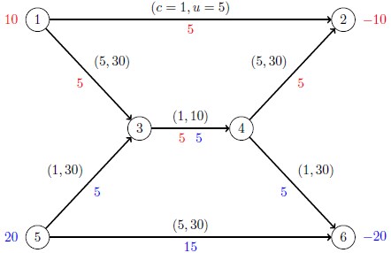
The optimal solution and solution summary are displayed in Output 15.1.1.
The optimal solution is shown on the network in Figure 15.6.
The iteration log, which contains the problem statistics, the progress of the solution, and the optimal objective value, is shown in Output 15.1.2.
Output 15.1.2: Log
| NOTE: There were 14 observations read from the data set WORK.ARC_COMM_DATA. |
| NOTE: There were 7 observations read from the data set WORK.ARC_DATA. |
| NOTE: There were 4 observations read from the data set WORK.SUPPLY_DATA. |
| NOTE: Problem generation will use 4 threads. |
| NOTE: The problem has 14 variables (0 free, 0 fixed). |
| NOTE: The problem has 19 linear constraints (7 LE, 12 EQ, 0 GE, 0 range). |
| NOTE: The problem has 42 linear constraint coefficients. |
| NOTE: The problem has 0 nonlinear constraints (0 LE, 0 EQ, 0 GE, 0 range). |
| NOTE: The LP presolver value NONE is applied. |
| NOTE: The LP solver is called. |
| NOTE: The Decomposition algorithm is used. |
| NOTE: The Decomposition algorithm is executing in single-machine mode. |
| NOTE: The DECOMP method value USER is applied. |
| NOTE: The problem has a decomposable structure with 2 blocks. The largest block covers 31.58% |
| of the constraints in the problem. |
| NOTE: The decomposition subproblems cover 14 (100.00%) variables and 12 (63.16%) constraints. |
| NOTE: The deterministic parallel mode is enabled. |
| NOTE: The Decomposition algorithm is using up to 4 threads. |
| Iter Best Master Gap CPU Real |
| Bound Objective Time Time |
| NOTE: Starting phase 1. |
| 1 0.0000 15.0000 1.50e+01 0.0 0.0 |
| 3 0.0000 0.0000 0.00% 0.0 0.0 |
| NOTE: Starting phase 2. |
| 4 150.0000 150.0000 0.00% 0.0 0.0 |
| NOTE: The Decomposition algorithm used 2 threads. |
| NOTE: The Decomposition algorithm time is 0.01 seconds. |
| NOTE: Optimal. |
| NOTE: Objective = 150. |