The Decomposition Algorithm
- Overview
-
Getting Started

-
SyntaxDecomposition Algorithm Options in the PROC OPTLP Statement or the SOLVE WITH LP Statement in PROC OPTMODELDecomposition Algorithm Options in the PROC OPTMILP Statement or the SOLVE WITH MILP Statement in PROC OPTMODELDECOMP StatementDECOMP_MASTER StatementDECOMP_MASTER_IP StatementDECOMP_SUBPROB Statement
-
Details
-
ExamplesMulticommodity Flow ProblemGeneralized Assignment ProblemBlock-Diagonal Structure and METHOD=AUTO in Single-Machine ModeBlock-Diagonal Structure and METHOD=AUTO in Distributed ModeBin Packing ProblemResource Allocation ProblemVehicle Routing ProblemATM Cash Management in Single-Machine ModeATM Cash Management in Distributed ModeKidney Donor Exchange
- References
This example describes an optimization model that is used in the management of cash flow for a bank’s automated teller machine (ATM) network. The goal of the model is to determine a replenishment schedule for the bank to use in allocating cash inventory at its branches when servicing a preassigned subset of ATMs. Given a history of withdrawals per day for each ATM, the bank can use SAS forecasting tools to predict the expected cash need. The modeling of this prediction depends on various seasonal factors, including the days of the week, weeks of the month, holidays, typical salary disbursement days, location of the ATMs, and other demographic data. The prediction is a parametric mixture of models whose parameters depend on each ATM.
The optimization model performs a polynomial regression that minimizes the error (measured by the ![]() norm) between the predicted and actual withdrawals. The parameter settings in the regression determine the replenishment
policy. The amount of cash that is allocated to each day is subject to a budget constraint. In addition, a constraint for
each ATM limits the number of days that a cash-out (a situation in which the cash flow is less than the predicted withdrawal) can occur. The goal is to determine a policy for
cash distribution that balances the predicted inventory levels while satisfying the budget and cash-out constraints. By keeping
too much cash on hand for ATM fulfillment, the bank loses an investment opportunity. Moreover, regulatory agencies in many
countries enforce a minimum cash reserve ratio at branch banks; according to regulatory policy, the cash in ATMs or in transit
does not contribute toward this threshold.
norm) between the predicted and actual withdrawals. The parameter settings in the regression determine the replenishment
policy. The amount of cash that is allocated to each day is subject to a budget constraint. In addition, a constraint for
each ATM limits the number of days that a cash-out (a situation in which the cash flow is less than the predicted withdrawal) can occur. The goal is to determine a policy for
cash distribution that balances the predicted inventory levels while satisfying the budget and cash-out constraints. By keeping
too much cash on hand for ATM fulfillment, the bank loses an investment opportunity. Moreover, regulatory agencies in many
countries enforce a minimum cash reserve ratio at branch banks; according to regulatory policy, the cash in ATMs or in transit
does not contribute toward this threshold.
The most natural formulation for this model is in the form of a mixed integer nonlinear program (MINLP). Let ![]() denote the set of ATMs and
denote the set of ATMs and ![]() denote the set of days that are used in the training data. The predictive model fit is defined by the following data for
each ATM
denote the set of days that are used in the training data. The predictive model fit is defined by the following data for
each ATM ![]() on each day
on each day ![]() :
: ![]() , and
, and ![]() . The model-fitting parameters define the variables
. The model-fitting parameters define the variables ![]() for each ATM that, when applied to the predictive model, estimate the necessary cash flow per day per ATM. In addition, define
a surrogate variable
for each ATM that, when applied to the predictive model, estimate the necessary cash flow per day per ATM. In addition, define
a surrogate variable ![]() for each ATM on each day that defines the cash inventory (replenished from the branch) minus withdrawals. The variable
for each ATM on each day that defines the cash inventory (replenished from the branch) minus withdrawals. The variable ![]() also represents the error in the regression model. Let
also represents the error in the regression model. Let ![]() define the budget per day,
define the budget per day, ![]() define the limit on cash-outs per ATM, and
define the limit on cash-outs per ATM, and ![]() define the historical withdrawals at a particular ATM on a particular day. Then the following MINLP models this problem:
define the historical withdrawals at a particular ATM on a particular day. Then the following MINLP models this problem:
![\begin{align*} & \text {minimize} & \sum _{a \in A} \sum _{d \in D} | f_{ad} | \\ & \text {subject to} & c^ x_{ad} x_{a} + c^ y_{ad} y_{a} + c^ z_{ad} x_{a} y_{a} + c^{u}_{ad} u_{a} + c_{ad} - w_{ad} & = f_{ad} & & a \in A,\ d \in D & & \text {(cash)}\\ & & \sum _{a \in A} \left(f_{ad} + w_{ad}\right) & \leq B_ d & & d \in D & & \text {(budget)}\\ & & | \{ d \in D \; | \; f_{ad} < 0\} | & \leq K_ a & & a \in A & & \text {(count)}\\ & & x_{a}, y_{a} & \in [0,1] & & a \in A \\ & & u_{a} & \geq 0 & & a \in A \\ & & f_{ad} & \geq -w_{ad} & & a \in A,\ d \in D \end{align*}](images/ormpug_decomp0134.png)
The cash constraint defines the surrogate variable ![]() , which gives the estimated net cash flow. The budget and count constraints ensure that the solution satisfies the budget
and cash-out constraints, respectively.
, which gives the estimated net cash flow. The budget and count constraints ensure that the solution satisfies the budget
and cash-out constraints, respectively.
To express this model in a more standard form, you can first use some standard model reformulations to linearize the absolute value and the cash-out constraint (count).
A well-known reformulation for linearizing the absolute value of a variable is to introduce one variable for each side of the absolute value. The following systems are equivalent:
|
|
is equivalent to |
![\[ \begin{array}{llll} \textrm{minimize} & y^+ + y^- \\ \textrm{subject to} & A (y^+ - y^-) & \leq & b \\ & y^+, y^- & \ge & 0 \end{array} \]](images/ormpug_decomp0136.png)
|
Let ![]() and
and ![]() represent the positive and negative parts, respectively, of the net cash flow
represent the positive and negative parts, respectively, of the net cash flow ![]() . Then you can rewrite the model, removing the absolute value, as the following:
. Then you can rewrite the model, removing the absolute value, as the following:
![\begin{align*} & \text {minimize} & \sum _{a \in A} \sum _{d \in D} \left(f^+_{ad} + f^-_{ad}\right) \\ & \text {subject to} & c^ x_{ad} x_{a} + c^ y_{ad} y_{a} + c^ z_{ad} x_{a} y_{a} + c^{u}_{ad} u_{a} + c_{ad} - w_{ad} & = f^+_{ad} - f^-_{ad} & & a \in A,\ d \in D \\ & & \sum _{a \in A} \left( f^+_{ad} - f^-_{ad} + w_{ad}\right) & \leq B_ d & & d \in D \\ & & | \{ d \in D \; | \; (f^{+}_{ad} - f^{-}_{ad}) < 0\} | & \leq K_ a & & a \in A \\ & & x_{a}, y_{a} & \in [0,1] & & a \in A\\ & & u_{a} & \geq 0 & & a \in A\\ & & f^+_{ad} & \geq 0 & & a \in A,\ d \in D\\ & & f^-_{ad} & \in [0,w_{ad}] & & a \in A,\ d \in D \end{align*}](images/ormpug_decomp0139.png)
To count the number of times a cash-out occurs, you need to introduce a binary variable to keep track of when this event
occurs. Let ![]() be an indicator variable that takes the value 1 when the net cash flow is negative. You can model the implication
be an indicator variable that takes the value 1 when the net cash flow is negative. You can model the implication ![]() , or its contrapositive
, or its contrapositive ![]() , by adding the constraint
, by adding the constraint
Now you can model the cash-out constraint by counting the number of days that the net-cash flow is negative for each ATM, as follows:
The MINLP model can now be written as follows:
![\begin{align*} & \text {minimize} & \sum _{a \in A} \sum _{d \in D} \left(f^+_{ad} + f^-_{ad}\right) \\ & \text {subject to} & c^ x_{ad} x_{a} + c^ y_{ad} y_{a} + c^ z_{ad} x_{a} y_{a} + c^{u}_{ad} u_{a} + c_{ad} - w_{ad} & = f^+_{ad} - f^-_{ad} & & a \in A,\ d \in D\\ & & \sum _{a \in A} \left(f^+_{ad} - f^-_{ad} + w_{ad} \right) & \leq B_ d & & d \in D\\ & & f^{-}_{ad} & \leq w_{ad} v_{ad} & & a \in A,\ d \in D\\ & & \sum _{ d \in D} v_{ad} & \leq K_ a & & a \in A\\ & & x_{a}, y_{a} & \in [0,1] & & a \in A\\ & & u_{a} & \geq 0 & & a \in A\\ & & f^+_{ad} & \geq 0 & & a \in A,\ d \in D \\ & & f^-_{ad} & \in [0,w_{ad}] & & a \in A,\ d \in D \\ & & v_{ad} & \in \{ 0,1\} & & a \in A,\ d \in D\\ \end{align*}](images/ormpug_decomp0145.png)
This MINLP is difficult to solve, in part because the prediction function is not convex. Another approach is to use mixed integer linear programming (MILP) to formulate an approximation of the problem, as described in the next section.
Because the predictive model is a forecast, finding the optimal parameters that are based on nondeterministic data is not
of primary importance. Rather, you want to provide as good a solution as possible in a reasonable amount of time. So using
MILP to approximate the MINLP is perfectly acceptable. In the original problem you have products of two continuous variables
that are both bounded by ![]() (lower bound) and
(lower bound) and ![]() (upper bound). This arrangement enables you to create an approximate linear model by using a few standard modeling reformulations.
(upper bound). This arrangement enables you to create an approximate linear model by using a few standard modeling reformulations.
The first step is to discretize one of the continuous variables ![]() . The goal is to transform the product
. The goal is to transform the product ![]() of a continuous variable and another continuous variable instead to the product of a continuous variable and a binary variable.
This transformation enables you to linearize the product form.
of a continuous variable and another continuous variable instead to the product of a continuous variable and a binary variable.
This transformation enables you to linearize the product form.
You must assume some level of approximation by defining a binary variable (from some discrete set) for each possible setting
of the continuous variable For example, if you let ![]() , then you allow
, then you allow ![]() to be chosen from the set
to be chosen from the set ![]() . Let
. Let ![]() represent the possible steps and
represent the possible steps and ![]() . Then you apply the following transformation to variable
. Then you apply the following transformation to variable ![]() :
:
The MINLP model can now be approximated as the following:
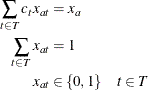
![\begin{align*} & \text {minimize} & \sum _{a \in A} \sum _{d \in D} \left(f^+_{ad} + f^-_{ad}\right) \\ & \text {subject to} & c^ x_{ad} \sum _{t \in T} c_ t x_{at} + c^ y_{ad} y_{a} + \\ & & c^ z_{ad} \sum _{t \in T} c_ t x_{at} y_{a} + c^{u}_{ad} u_{a} + c_{ad} - w_{ad} & = f^+_{ad} - f^-_{ad} & & a \in A,\ d \in D \\ & & \sum _{t \in T} x_{at} & = 1 & & a \in A \\ & & \sum _{a \in A} \left(f^+_{ad} - f^-_{ad} + w_{ad} \right) & \leq B_ d & & d \in D\\ & & f^{-}_{ad} & \leq w_{ad} v_{ad} & & a \in A,\ d \in D \\ & & \sum _{ d \in D} v_{ad} & \leq K_ a & & a \in A\\ & & y_{a} & \in [0,1] & & a \in A\\ & & u_{a} & \geq 0 & & a \in A \\ & & f^+_{ad} & \geq 0 & & a \in A,\ d \in D\\ & & f^-_{ad} & \in [0,w_{ad}] & & a \in A,\ d \in D\\ & & v_{ad} & \in \{ 0,1\} & & a \in A,\ d \in D\\ & & x_{at} & \in \{ 0,1\} & & a \in A,\ t \in T \end{align*}](images/ormpug_decomp0155.png)
You still need to linearize the product terms ![]() in the cash flow constraint. Because these terms are products of a bounded continuous variable and a binary variable, you
can linearize them by introducing for each product another variable,
in the cash flow constraint. Because these terms are products of a bounded continuous variable and a binary variable, you
can linearize them by introducing for each product another variable, ![]() , which serves as a surrogate. In general, you know the following relationship between the original variables and their surrogates:
, which serves as a surrogate. In general, you know the following relationship between the original variables and their surrogates:
|
![\[ \begin{array}{lcll} z_ t & = & x_ t y & t \in T \\ \sum _{t \in T} x_{t} & = & 1 \\ x_ t & \in & \{ 0,1\} & t \in T \\ y & \in & [0,1] \end{array} \]](images/ormpug_decomp0158.png)
is equivalent to
![\[ \begin{array}{lcll} z_ t & \ge & 0 & t \in T\\ z_ t & \le & x_ t & t \in T\\ \sum _{t \in T} x_{t} & = & 1 \\ \sum _{t \in T} z_{t} & = & y \\ x_ t & \in & \{ 0,1\} & t \in T \\ y & \in & [0,1] \end{array} \]](images/ormpug_decomp0159.png)
|
Using this relationship to replace each product form, you now can write the problem as an approximate MILP as follows:
![\begin{align*} & \text {minimize} & \sum _{a \in A} \sum _{d \in D} \left( f^+_{ad} + f^-_{ad}\right) \\ & \text {subject to} & c^ x_{ad} \sum _{t \in T} c_ t x_{at} + c^ y_{ad} y_{a} + \\ & & c^ z_{ad} \sum _{t \in T} c_ t z_{at} + c^{u}_{ad} u_{a} + c_{ad} - w_{ad} & = f^+_{ad} - f^-_{ad} & & a \in A,\ d \in D \\ & & \sum _{t \in T} x_{at} & = 1 & & a \in A\\ & & \sum _{a \in A} \left(f^+_{ad} - f^-_{ad} + w_{ad} \right) & \leq B_ d & & d \in D & & \text {(budget)}\\ & & f^{-}_{ad} & \leq w_{ad} v_{ad} & & a \in A,\ d \in D\\ & & \sum _{ d \in D} v_{ad} & \leq K_ a & & a \in A\\ & & z_{at} & \leq x_{at} & & a \in A,\ t \in T\\ & & \sum _{t \in T} z_{at} & = y_{a} & & a \in A\\ & & z_{at} & \geq 0 & & a \in A,\ t \in T\\ & & y_{a} & \in [0,1] & & a \in A\\ & & u_{a} & \geq 0 & & a \in A\\ & & f^+_{ad} & \geq 0 & & a \in A,\ d \in D\\ & & f^-_{ad} & \in [0,w_{ad}] & & a \in A,\ d \in D\\ & & v_{ad} & \in \{ 0,1\} & & a \in A,\ d \in D\\ & & x_{at} & \in \{ 0,1\} & & a \in A,\ t \in T \end{align*}](images/ormpug_decomp0160.png)
Because it is difficult to solve the MINLP model directly, the approximate MILP formulation is attractive. Unfortunately, the approximate MILP is much larger than the associated MINLP. Direct methods for solving this MILP do not work well. However, the problem is nicely suited for the decomposition algorithm.
When you examine the structure of the MILP model, you see clearly that the constraints can be easily decomposed by ATM. In fact, the only set of constraints that involve decision variables across ATMs is the budget constraint (budget). That is, if you relax the budget constraint, you are left with independent blocks of constraints, one for each ATM.
To show how this is done in PROC OPTMODEL, consider the following data sets, which describe an example that tracks 20 ATMs over a period of 100 days. This particular example was submitted to MIPLIB 2010, which is a collection of difficult MILPs in the public domain (Koch et al., 2011).
The first data set, budget_data, provides the cash budget on each particular day:
data budget_data;
   input d $ budget;
   datalines;
DATE0      70079
DATE1      66418
DATE10     52656
DATE11     50439
DATE12     58688
DATE13     45002
DATE14     52369
...
;
The second data set, cashout_data, provides the limit on the number of cash-outs that are allowed at each ATM:
data cashout_data;
   input a $ cashOutLimit;
   datalines;
ATM0            31
ATM1            24
ATM2            41
ATM3            43
ATM4            29
ATM5            24
ATM6            52
ATM7            44
ATM8            35
ATM9            48
ATM10           31
ATM11           47
ATM12           26
ATM13           34
ATM14           29
ATM15           32
ATM16           33
ATM17           32
ATM18           43
ATM19           28
;
The final data set, polyfit_data, provides the polynomial fit coefficients for each ATM on each date. It also provides the historical cash withdrawals.
data polyfit_data;
   input a $ d $ cx cy cz cu c withdrawal;
   datalines;
ATM0     DATE0       2822     1984    -1984    1045    1373        780
ATM0     DATE1       1337     2530    -2530    1510     174       2351
ATM0     DATE2       2685      -67       67     145    2820       2288
ATM0     DATE3       -595    -3135     3135     581    3319       1357
...
ATM19    DATE96      -734     3392    -3392     162    1648        914
ATM19    DATE97     -1062      969     -969     444    1746       2264
ATM19    DATE98      7676     2308    -2308      59    1388        972
ATM19    DATE99      3062     1308    -1308    1080     654        698
;
The following PROC OPTMODEL statements read in the data and define the necessary sets and parameters:
proc optmodel;
   set<str> DATES;
   set<str> ATMS;

   /* cash budget per date */
   num budget{DATES};

   /* maximum number of cash-outs allowed at each atm */
   num cashOutLimit{ATMS};

   /* historical withdrawal amount per atm each date */
   num withdrawal{ATMS, DATES};

   /* polynomial fit coefficients for predicted cash flow needed */
   num c {ATMS, DATES};
   num cx{ATMS, DATES};
   num cy{ATMS, DATES};
   num cz{ATMS, DATES};
   num cu{ATMS, DATES};

   /* number of points used in approximation of continuous range */
   num nSteps = 10;
   set STEPS = {0..nSteps};

   read data budget_data into DATES=[d] budget;
   read data cashout_data into ATMS=[a] cashOutLimit;
   read data polyfit_data into [a d] cx cy cz cu c withdrawal;
The following statements declare the variables:
   var x{ATMS,STEPS}                 binary;
   var v{ATMS,DATES}                 binary;
   var z{ATMS,STEPS}                 >= 0 <= 1;
   var y{ATMS}                       >= 0 <= 1;
   var u{ATMS}                       >= 0;
   var fPlus{ATMS,DATES}             >= 0;
   var fMinus{a in ATMS, d in DATES} >= 0 <= withdrawal[a,d];
The following statements declare the objective and the constraints:
   min CashFlowDiff =
      sum{a in ATMS, d in DATES} (fPlus[a,d] + fMinus[a,d]);

   con BudgetCon{d in DATES}:
      sum{a in ATMS} (fPlus[a,d] - fMinus[a,d] + withdrawal[a,d])
          <= budget[d];

   con CashFlowDefCon{a in ATMS, d in DATES}:
      cx[a,d] * sum{t in STEPS} (t/nSteps) * x[a,t] +
      cy[a,d] * y[a]                                +
      cz[a,d] * sum{t in STEPS} (t/nSteps) * z[a,t] +
      cu[a,d] * u[a]                                +
      c[a,d] - withdrawal[a,d] = fPlus[a,d] - fMinus[a,d];

   con PickOneStepCon{a in ATMS}:
      sum{t in STEPS} x[a,t] = 1;

   con CashOutLinkCon{a in ATMS, d in DATES}:
      fMinus[a,d] <= withdrawal[a,d] * v[a,d];

   con CashOutLimitCon{a in ATMS}:
      sum{d in DATES} v[a,d] <= cashOutLimit[a];

   con Linear1Con{a in ATMS, t in STEPS}:
      z[a,t] <= x[a,t];

   con Linear2Con{a in ATMS}:
      sum{t in STEPS} z[a,t] = y[a];
The following statements define the block decomposition by ATM. The .block suffix expects numeric indices, whereas the SET<STR> ATMS statement declares a set of strings. You can create a mapping from the string identifier to a numeric identifier as follows:
   /* create numeric block index */
   num blockIndex {ATMS};
   num index init 0;
   for{a in ATMS} do;
      blockIndex[a] = index;
      index = index + 1;
   end;
Then, each constraint can be added to its associated ATM block as follows:
   /* define blocks for each ATM */
   for{a in ATMS} do;
      PickOneStepCon[a].block  = blockIndex[a];
      CashOutLimitCon[a].block = blockIndex[a];
      Linear2Con[a].block      = blockIndex[a];
      for{d in DATES} do;
         CashFlowDefCon[a,d].block = blockIndex[a];
         CashOutLinkCon[a,d].block = blockIndex[a];
      end;
      for{t in STEPS} do;
         Linear1Con[a,t].block = blockIndex[a];
      end;
   end;
The budget constraint links all the ATMs, and it remains in the master problem. Finally, the following statements use DECOMP to solve the problem:
   /* set the number of threads and get performance details */
   performance details nthreads=4;

   /* solve with the decomposition algorithm */
   solve with milp / decomp=();
quit;
The solution summary, performance information, and procedure task timing tables are displayed in Output 14.8.1.
Output 14.8.1: Performance Information, Solution Summary, and Task Timing Tables
| Performance Information | |
|---|---|
| Execution Mode | Single-Machine |
| Number of Threads | 4 |
| Solution Summary | |
|---|---|
| Solver | MILP |
| Algorithm | Decomposition |
| Objective Function | CashFlowDiff |
| Solution Status | Optimal within Relative Gap |
| Objective Value | 2463699.6896 |
| Relative Gap | 0.0000626319 |
| Absolute Gap | 154.2964477 |
| Primal Infeasibility | 1.828084E-10 |
| Bound Infeasibility | 0 |
| Integer Infeasibility | 3.663736E-15 |
| Best Bound | 2463545.3932 |
| Nodes | 14 |
| Iterations | 22 |
| Presolve Time | 0.20 |
| Solution Time | 199.05 |
| Procedure Task Timing | ||
|---|---|---|
| Task | Time (sec.) |
% Time |
| Problem Generation | 0.04 | 0.02% |
| Solver Initialization | 0.07 | 0.04% |
| Code Generation | 0.00 | 0.00% |
| Solver | 199.06 | 99.94% |
| Solver Postprocessing | 0.01 | 0.00% |
The iteration log, which contains the problem statistics, the progress of the solution, and the optimal objective value, is shown in Output 14.8.2.
Output 14.8.2: Log
| NOTE: There were 100 observations read from the data set WORK.BUDGET_DATA. |
| NOTE: There were 20 observations read from the data set WORK.CASHOUT_DATA. |
| NOTE: There were 2000 observations read from the data set WORK.POLYFIT_DATA. |
| NOTE: Problem generation will use 4 threads. |
| NOTE: The problem has 6480 variables (0 free, 0 fixed). |
| NOTE: The problem has 2220 binary and 0 integer variables. |
| NOTE: The problem has 4380 linear constraints (2340 LE, 2040 EQ, 0 GE, 0 range). |
| NOTE: The problem has 58878 linear constraint coefficients. |
| NOTE: The problem has 0 nonlinear constraints (0 LE, 0 EQ, 0 GE, 0 range). |
| NOTE: The MILP presolver value AUTOMATIC is applied. |
| NOTE: The MILP presolver removed 502 variables and 345 constraints. |
| NOTE: The MILP presolver removed 1172 constraint coefficients. |
| NOTE: The MILP presolver modified 0 constraint coefficients. |
| NOTE: The presolved problem has 5978 variables, 4035 constraints, and 57706 |
| constraint coefficients. |
| NOTE: The MILP solver is called. |
| NOTE: The Decomposition algorithm is used. |
| NOTE: The Decomposition algorithm is executing in single-machine mode. |
| NOTE: The DECOMP method value USER is applied. |
| NOTE: The problem has a decomposable structure with 20 blocks. The largest block |
| covers 5.18% of the constraints in the problem. |
| NOTE: The decomposition subproblems cover 5978 (100.00%) variables and 3935 (97.52%) |
| constraints. |
| NOTE: The deterministic parallel mode is enabled. |
| NOTE: The Decomposition algorithm is using up to 4 threads. |
| Iter Best Master Best LP IP CPU Real |
| Bound Objective Integer Gap Gap Time Time |
| NOTE: Starting phase 1. |
| 1 0.0000 1.1767 . 1.18e+00 . 91 28 |
| 2 0.0000 0.0000 . 0.00% . 91 28 |
| NOTE: Starting phase 2. |
| . 2.4432e+06 2.6798e+06 2.7511e+06 9.69% 12.60% 91 29 |
| 4 2.4526e+06 2.4833e+06 2.7511e+06 1.25% 12.17% 160 49 |
| 5 2.4630e+06 2.4642e+06 2.7511e+06 0.05% 11.70% 196 59 |
| NOTE: The Decomposition algorithm stopped on the continuous RELOBJGAP= option. |
| . 2.4630e+06 2.4632e+06 2.4775e+06 0.01% 0.59% 196 59 |
| 6 2.4630e+06 2.4632e+06 2.4775e+06 0.01% 0.59% 196 59 |
| NOTE: Starting branch and bound. |
| Node Active Sols Best Best Gap CPU Real |
| Integer Bound Time Time |
| 0 1 2 2.4775e+06 2.4630e+06 0.59% 196 59 |
| 10 10 3 2.4654e+06 2.4635e+06 0.07% 542 166 |
| 13 5 4 2.4637e+06 2.4635e+06 0.01% 640 196 |
| NOTE: The Decomposition algorithm used 4 threads. |
| NOTE: The Decomposition algorithm time is 196.27 seconds. |
| NOTE: Optimal within relative gap. |
| NOTE: Objective = 2463699.6896. |