The Decomposition Algorithm
- Overview
-
Getting Started

-
SyntaxDecomposition Algorithm Options in the PROC OPTLP Statement or the SOLVE WITH LP Statement in PROC OPTMODELDecomposition Algorithm Options in the PROC OPTMILP Statement or the SOLVE WITH MILP Statement in PROC OPTMODELDECOMP StatementDECOMP_MASTER StatementDECOMP_MASTER_IP StatementDECOMP_SUBPROB Statement
-
Details
-
ExamplesMulticommodity Flow ProblemGeneralized Assignment ProblemBlock-Diagonal Structure and METHOD=AUTO in Single-Machine ModeBlock-Diagonal Structure and METHOD=AUTO in Distributed ModeBin Packing ProblemResource Allocation ProblemVehicle Routing ProblemATM Cash Management in Single-Machine ModeATM Cash Management in Distributed ModeKidney Donor Exchange
- References
This example describes a model for selecting tasks to be run on a shared resource (Gamrath, 2010). Consider a set ![]() of tasks and a resource capacity
of tasks and a resource capacity ![]() . Each item
. Each item ![]() has a profit
has a profit ![]() , a resource utilization level
, a resource utilization level ![]() , a starting period
, a starting period ![]() , and an ending period
, and an ending period ![]() . The time horizon considered is from the earliest starting time to the latest ending time of all tasks. With each task, associate
a binary variable
. The time horizon considered is from the earliest starting time to the latest ending time of all tasks. With each task, associate
a binary variable ![]() , which, if set to
, which, if set to ![]() , indicates that the task is running from its start time until just before its end time. A task consumes capacity if it is
running. The goal is to select which tasks to run in order to maximize profit while not exceeding the shared resource capacity.
Let
, indicates that the task is running from its start time until just before its end time. A task consumes capacity if it is
running. The goal is to select which tasks to run in order to maximize profit while not exceeding the shared resource capacity.
Let ![]() define the set of start times for all tasks, and let
define the set of start times for all tasks, and let ![]() define the set of tasks that are running at each start time
define the set of tasks that are running at each start time ![]() . The problem can be modeled as a mixed integer linear programming problem as follows:
. The problem can be modeled as a mixed integer linear programming problem as follows:
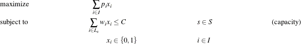
In this formulation, constraints (capacity) ensure that the running tasks do not exceed the resource capacity. To illustrate,
consider the following five-task example with data: ![]() ,
, ![]() ,
, ![]() ,
, ![]() , and
, and ![]() . The formulation leads to a constraint matrix that has a staircase structure that is determined by tasks coming on and offline:
. The formulation leads to a constraint matrix that has a staircase structure that is determined by tasks coming on and offline:
![\[ \begin{array}{rlllllllllll} \mbox{maximize} & 6 x_1 & + & 8 x_2 & + & 5 x_3 & + & 9 x_4 & + & 8 x_5 \\ \mbox{subject to} & 8 x_1 & & & & & & & & & \leq & 10 \\ & 8 x_1 & + & 5 x_2 & & & & & & & \leq & 10 \\ & & & 5 x_2 & + & 3 x_3 & & & & & \leq & 10 \\ & & & 5 x_2 & + & 3 x_3 & + & 4 x_4 & & & \leq & 10 \\ & & & & + & 3 x_3 & + & 4 x_4 & + & 3 x_5 & \leq & 10 \\ & \multicolumn{11}{l}{x_ i \in \{ 0,1\} \quad i \in I}\\ \end{array} \]](images/ormpug_decomp0097.png)
This formulation clearly has no decomposable structure. However, you can use a common modeling technique known as Lagrangian decomposition to bring the model into block-angular form. Lagrangian decomposition works by first partitioning the constraints into blocks. Then, each original variable is split into multiple copies of itself, one copy for each block in which the variable has a nonzero coefficient in the constraint matrix. Constraints are added to enforce the equality of each copy of the original variable. Then, the original constraints can be written in block-angular form by using the duplicate variables.
To apply Lagrangian decomposition to the resource allocation problem, define a set ![]() of blocks and let
of blocks and let ![]() define the set of start times for a given block
define the set of start times for a given block ![]() , such that
, such that ![]() . Given this partition of start times, let
. Given this partition of start times, let ![]() define the set of blocks in which task
define the set of blocks in which task ![]() is scheduled to be running. Now, for each task
is scheduled to be running. Now, for each task ![]() , define duplicate variables
, define duplicate variables ![]() for each
for each ![]() . Let
. Let ![]() define the minimum block index for each class of variable that represents task
define the minimum block index for each class of variable that represents task ![]() . The problem can now be modeled in block-angular form as follows:
. The problem can now be modeled in block-angular form as follows:
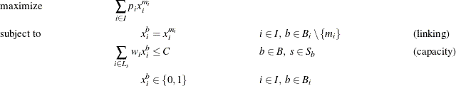
In this formulation, constraints (linking) ensure that the duplicate variables are equal to the original variables. Now, the five-task example has been transformed from a staircase structure to a block-angular structure:
![\[ \begin{array}{r*{18}{r}} \mbox{maximize} & 6 x_1^1 & + & 8 x_2^1 & + & & & 5 x_3^2 & + & 9 x_4^2 & + & & & & & 8 x_5^3 \\ \mbox{subject to} & & & x_2^1 & - & x_2^2 & & & & & & & & & & & = & 0 \\ & & & & & & & x_3^2 & - & & & x_3^3 & & & & & = & 0 \\ & & & & & & & & & x_4^2 & & & - & x_4^3 & & & = & 0 \\ & 8 x_1^1 & & & & & & & & & & & & & & & \leq & 10 \\ & 8 x_1^1 & + & 5 x_2^1 & & & & & & & & & & & & & \leq & 10 \\ & & & & & 5 x_2^2 & + & 3 x_3^2 & & & & & & & & & \leq & 10 \\ & & & & & 5 x_2^2 & + & 3 x_3^2 & + & 4 x_4^2 & & & & & & & \leq & 10 \\ & & & & & & & & & & & 3 x_3^3 & + & 4 x_4^3 & + & 3 x_5^3 & \leq & 10 \\ & \multicolumn{11}{l}{x_ i^ b \in \{ 0,1\} \quad i \in I, \ b \in B_ i}\\ \end{array} \]](images/ormpug_decomp0106.png)
To show how to apply Lagrangian decomposition
in PROC OPTMODEL, consider the following data set TaskData from Caprara, Furini, and Malaguti (2010) which consists of ![]() tasks:
tasks:
data TaskData;
   input profit weight start end;
   datalines;
100 74    1   12
 98 32    1    9
 73 27    1   22
 98 51    1   31
...
 23 40 2684 2689
 36 85 2685 2687
 65 44 2686 2689
 18 36 2687 2689
 88 57 2688 2689
;
The following PROC OPTMODEL statements read in the data and solve the original staircase formulation by calling the MILP solver directly:
%macro SetupData(task_data=, capacity=);
   set TASKS;
   num capacity=&capacity;
   num profit{TASKS}, weight{TASKS}, start{TASKS}, end{TASKS};

   read data &task_data into TASKS=[_n_] profit weight start end;
   /* the set of start times */

   set STARTS = setof{i in TASKS} start[i];
   /* the set of tasks i that are active at a given start time s */
   set TASKS_START{s in STARTS}
      = {i in TASKS: start[i] <= s < end[i]};
%mend SetupData;

%macro ResourceAllocation_Direct(task_data=, capacity=);
   proc optmodel;
      %SetupData(task_data=&task_data,capacity=&capacity);

      /* select task i to come online from period [start to end) */
      var x{TASKS} binary;

      /* maximize the total profit of running tasks */
      max TotalProfit = sum{i in TASKS} profit[i] * x[i];

      /* enforce that the shared resource capacity is not exceeded */
      con CapacityCon{s in STARTS}:
         sum{i in TASKS_START[s]} weight[i] * x[i] <= capacity;

      solve;
   quit;
%mend ResourceAllocation_Direct;

%ResourceAllocation_Direct(task_data=TaskData, capacity=100);
The problem summary and solution summary are displayed in Output 14.6.1.
Output 14.6.1: Problem Summary and Solution Summary
| Problem Summary | |
|---|---|
| Objective Sense | Maximization |
| Objective Function | TotalProfit |
| Objective Type | Linear |
| Number of Variables | 2697 |
| Bounded Above | 0 |
| Bounded Below | 0 |
| Bounded Below and Above | 2697 |
| Free | 0 |
| Fixed | 0 |
| Binary | 2697 |
| Integer | 0 |
| Number of Constraints | 2688 |
| Linear LE (<=) | 2688 |
| Linear EQ (=) | 0 |
| Linear GE (>=) | 0 |
| Linear Range | 0 |
| Constraint Coefficients | 26880 |
| Solution Summary | |
|---|---|
| Solver | MILP |
| Algorithm | Branch and Cut |
| Objective Function | TotalProfit |
| Solution Status | Optimal within Relative Gap |
| Objective Value | 62520 |
| Relative Gap | 0.000094456 |
| Absolute Gap | 5.9059496407 |
| Primal Infeasibility | 0 |
| Bound Infeasibility | 0 |
| Integer Infeasibility | 0 |
| Best Bound | 62525.90595 |
| Nodes | 319 |
| Iterations | 14124 |
| Presolve Time | 0.59 |
| Solution Time | 36.50 |
The iteration log, which contains the problem statistics, the progress of the solution, and the optimal objective value, is shown in Output 14.6.2.
Output 14.6.2: Log
| NOTE: There were 2697 observations read from the data set WORK.TASKDATA. |
| NOTE: Problem generation will use 4 threads. |
| NOTE: The problem has 2697 variables (0 free, 0 fixed). |
| NOTE: The problem has 2697 binary and 0 integer variables. |
| NOTE: The problem has 2688 linear constraints (2688 LE, 0 EQ, 0 GE, 0 range). |
| NOTE: The problem has 26880 linear constraint coefficients. |
| NOTE: The problem has 0 nonlinear constraints (0 LE, 0 EQ, 0 GE, 0 range). |
| NOTE: The OPTMODEL presolver is disabled for linear problems. |
| NOTE: The MILP presolver value AUTOMATIC is applied. |
| NOTE: The MILP presolver removed 0 variables and 0 constraints. |
| NOTE: The MILP presolver removed 0 constraint coefficients. |
| NOTE: The MILP presolver modified 0 constraint coefficients. |
| NOTE: The presolved problem has 2697 variables, 2688 constraints, and 26880 |
| constraint coefficients. |
| NOTE: The MILP solver is called. |
| Node Active Sols BestInteger BestBound Gap Time |
| 0 1 3 54182.0000000 145710 62.82% 0 |
| 0 1 3 54182.0000000 73230.2096818 26.01% 0 |
| 0 1 6 60619.0000000 70137.4443874 13.57% 1 |
| 0 1 7 61212.0000000 68400.8103508 10.51% 2 |
| 0 1 7 61212.0000000 67050.7090333 8.71% 2 |
| 0 1 7 61212.0000000 66009.5116948 7.27% 3 |
| 0 1 7 61212.0000000 65136.9326305 6.03% 4 |
| 0 1 7 61212.0000000 64537.6386548 5.15% 4 |
| 0 1 7 61212.0000000 64102.6120406 4.51% 5 |
| 0 1 7 61212.0000000 63810.6627587 4.07% 5 |
| 0 1 7 61212.0000000 63608.5446906 3.77% 5 |
| 0 1 7 61212.0000000 63409.6302212 3.47% 5 |
| 0 1 7 61212.0000000 63285.7987214 3.28% 5 |
| 0 1 7 61212.0000000 63200.2587270 3.15% 5 |
| 0 1 7 61212.0000000 63115.8950073 3.02% 5 |
| 0 1 7 61212.0000000 63063.8727915 2.94% 5 |
| 0 1 7 61212.0000000 63001.7922826 2.84% 5 |
| 0 1 7 61212.0000000 62957.3490752 2.77% 5 |
| 0 1 7 61212.0000000 62923.1614916 2.72% 5 |
| 0 1 7 61212.0000000 62903.4110327 2.69% 5 |
| 0 1 7 61212.0000000 62879.2339594 2.65% 6 |
| 0 1 7 61212.0000000 62866.5588746 2.63% 6 |
| 0 1 7 61212.0000000 62854.8930615 2.61% 6 |
| 0 1 7 61212.0000000 62842.9466737 2.60% 6 |
| 0 1 7 61212.0000000 62830.2710225 2.58% 6 |
| 0 1 7 61212.0000000 62822.2853239 2.56% 6 |
| 0 1 7 61212.0000000 62818.0708084 2.56% 6 |
| 0 1 8 61294.0000000 62818.0708084 2.43% 6 |
| 0 1 8 61294.0000000 62818.0708084 2.43% 6 |
| NOTE: The MILP solver added 1295 cuts with 8693 cut coefficients at the root. |
| 42 41 9 61384.0000000 62797.0665836 2.25% 12 |
| 63 61 13 62417.0000000 62784.3661896 0.59% 15 |
| 100 97 13 62417.0000000 62777.3661896 0.57% 20 |
| 147 98 16 62494.0000000 62751.8640081 0.41% 29 |
| 163 95 17 62520.0000000 62741.4776445 0.35% 32 |
| 200 89 17 62520.0000000 62604.5430948 0.14% 34 |
| 300 38 17 62520.0000000 62531.9156776 0.02% 36 |
| 318 22 17 62520.0000000 62525.9059496 0.01% 36 |
| NOTE: Optimal within relative gap. |
| NOTE: Objective = 62520. |
To transform this data into block-angular form, first sort the task data to help reduce the number of duplicate variables needed in the reformulation as follows:
proc sort data=TaskData;
   by start end;
run;
Then, create the partition of constraints into blocks of size block_size as follows:
%macro ResourceAllocation_Decomp(task_data=, capacity=, block_size=);
   proc optmodel;
      %SetupData(task_data=&task_data,capacity=&capacity);
      /* partition into blocks of size blocks_size */
      num block_size = &block_size;
      num num_blocks = ceil( card(TASKS) / block_size );
      set BLOCKS     = 1..num_blocks;

      /* the set of starts s for which task i is active */
      set STARTS_TASK{i in TASKS} = {s in STARTS: start[i] <= s < end[i]};

      /* partition the start times into blocks of size block_size */
      set STARTS_BLOCK{BLOCKS} init {};
      num block_id    init 1;
      num block_count init 0;
      for{s in STARTS} do;
         STARTS_BLOCK[block_id] = STARTS_BLOCK[block_id] union {s};
         block_count = block_count + 1;
         if(mod(block_count, block_size) = 0) then
             block_id = block_id + 1;
      end;
Then, the following PROC OPTMODEL statements define the block-angular formulation and solve the problem by using the decomposition
algorithm, the PRESOLVER=BASIC option, and block_size=40. Because this reformulation is equivalent to the original staircase formulation, disabling some of the advanced presolver
techniques ensures that the model maintains block-angularity.
      /* blocks in which task i is online */
      set BLOCKS_TASK{i in TASKS} =
         {b in BLOCKS: card(STARTS_BLOCK[b] inter STARTS_TASK[i]) > 0};

      /* minimum block id in which task i is online */
      num min_block{i in TASKS} = min{b in BLOCKS_TASK[i]} b;

      /* select task i to come online from period [start to end)
         in each block */
      var x{i in TASKS, b in BLOCKS_TASK[i]} binary;

      /* maximize the total profit of running tasks */
      max TotalProfit = sum{i in TASKS} profit[i] * x[i,min_block[i]];

      /* enforce that task selection is consistent across blocks */
      con LinkDupVarsCon{i in TASKS, b in BLOCKS_TASK[i] diff {min_block[i]}}:
         x[i,b] = x[i,min_block[i]];

      /* enforce that the shared resource capacity is not exceeded */
      con CapacityCon{b in BLOCKS, s in STARTS_BLOCK[b]}:
         sum{i in TASKS_START[s]} weight[i] * x[i,b] <= capacity;

      /* define blocks for decomposition algorithm */
      for{b in BLOCKS, s in STARTS_BLOCK[b]} CapacityCon[b,s].block = b;

      solve with milp / presolver=basic decomp=();
   quit;
%mend ResourceAllocation_Decomp;

%ResourceAllocation_Decomp(task_data=TaskData, capacity=100, block_size=40);
The problem summary and solution summary are displayed in Output 14.6.3. Compared to the original formulation, the number of variables and constraints is increased by the number of duplicate variables.
Output 14.6.3: Problem Summary and Solution Summary
| Problem Summary | |
|---|---|
| Objective Sense | Maximization |
| Objective Function | TotalProfit |
| Objective Type | Linear |
| Number of Variables | 3300 |
| Bounded Above | 0 |
| Bounded Below | 0 |
| Bounded Below and Above | 3300 |
| Free | 0 |
| Fixed | 0 |
| Binary | 3300 |
| Integer | 0 |
| Number of Constraints | 3291 |
| Linear LE (<=) | 2688 |
| Linear EQ (=) | 603 |
| Linear GE (>=) | 0 |
| Linear Range | 0 |
| Constraint Coefficients | 28086 |
| Solution Summary | |
|---|---|
| Solver | MILP |
| Algorithm | Decomposition |
| Objective Function | TotalProfit |
| Solution Status | Optimal within Relative Gap |
| Objective Value | 62524 |
| Relative Gap | 0.0000693019 |
| Absolute Gap | 4.3333333333 |
| Primal Infeasibility | 2.220446E-16 |
| Bound Infeasibility | 8.881784E-16 |
| Integer Infeasibility | 9.992007E-16 |
| Best Bound | 62528.333333 |
| Nodes | 4 |
| Iterations | 42 |
| Presolve Time | 1.08 |
| Solution Time | 22.05 |
The iteration log, which contains the problem statistics, the progress of the solution, and the optimal objective value, is shown in Output 14.6.4.
Output 14.6.4: Log
| NOTE: There were 2697 observations read from the data set WORK.TASKDATA. |
| NOTE: Problem generation will use 4 threads. |
| NOTE: The problem has 3300 variables (0 free, 0 fixed). |
| NOTE: The problem has 3300 binary and 0 integer variables. |
| NOTE: The problem has 3291 linear constraints (2688 LE, 603 EQ, 0 GE, 0 range). |
| NOTE: The problem has 28086 linear constraint coefficients. |
| NOTE: The problem has 0 nonlinear constraints (0 LE, 0 EQ, 0 GE, 0 range). |
| NOTE: The MILP presolver value BASIC is applied. |
| NOTE: The MILP presolver removed 0 variables and 0 constraints. |
| NOTE: The MILP presolver removed 0 constraint coefficients. |
| NOTE: The MILP presolver modified 0 constraint coefficients. |
| NOTE: The presolved problem has 3300 variables, 3291 constraints, and 28086 |
| constraint coefficients. |
| NOTE: The MILP solver is called. |
| NOTE: The Decomposition algorithm is used. |
| NOTE: The Decomposition algorithm is executing in single-machine mode. |
| NOTE: The DECOMP method value USER is applied. |
| NOTE: The problem has a decomposable structure with 68 blocks. The largest block |
| covers 1.22% of the constraints in the problem. |
| NOTE: The decomposition subproblems cover 3300 (100.00%) variables and 2688 (81.68%) |
| constraints. |
| NOTE: The deterministic parallel mode is enabled. |
| NOTE: The Decomposition algorithm is using up to 4 threads. |
| Iter Best Master Best LP IP CPU Real |
| Bound Objective Integer Gap Gap Time Time |
| NOTE: Starting phase 1. |
| 1 0.0000 0.0000 . 0.00% . 1 0 |
| NOTE: Starting phase 2. |
| . 65890.0000 54109.0000 54109.0000 17.88% 17.88% 1 0 |
| 3 65890.0000 55585.0000 55585.0000 15.64% 15.64% 3 1 |
| 4 65890.0000 56635.5000 56605.0000 14.05% 14.09% 4 1 |
| 5 65890.0000 59076.0000 58832.0000 10.34% 10.71% 5 1 |
| 6 65890.0000 59909.0000 59878.0000 9.08% 9.12% 6 2 |
| 7 65890.0000 60662.5000 60552.0000 7.93% 8.10% 8 2 |
| 8 65890.0000 61207.5000 61017.0000 7.11% 7.40% 9 3 |
| 9 65890.0000 61722.4333 61522.0000 6.33% 6.63% 11 3 |
| . 65890.0000 61875.3333 61868.0000 6.09% 6.10% 11 3 |
| 10 65259.3333 61875.3333 61868.0000 5.19% 5.20% 12 4 |
| 11 64963.8889 61997.0000 61962.0000 4.57% 4.62% 14 4 |
| 12 63897.0833 62406.0000 62386.0000 2.33% 2.36% 15 5 |
| 13 63314.0833 62445.0000 62445.0000 1.37% 1.37% 17 5 |
| 14 63096.5333 62460.3333 62445.0000 1.01% 1.03% 18 6 |
| 15 62789.0476 62493.3333 62476.0000 0.47% 0.50% 20 7 |
| 16 62789.0476 62494.3333 62477.0000 0.47% 0.50% 22 7 |
| 17 62657.3333 62501.3333 62477.0000 0.25% 0.29% 24 8 |
| 18 62655.2500 62501.3333 62477.0000 0.25% 0.28% 25 8 |
| 19 62608.3333 62501.3333 62477.0000 0.17% 0.21% 27 9 |
| . 62608.3333 62516.6667 62477.0000 0.15% 0.21% 27 9 |
| 20 62558.6667 62516.6667 62477.0000 0.07% 0.13% 29 10 |
| 24 62528.3333 62524.3333 62477.0000 0.01% 0.08% 35 12 |
| NOTE: The Decomposition algorithm stopped on the continuous RELOBJGAP= option. |
| 24 62528.3333 62524.3333 62477.0000 0.01% 0.08% 35 12 |
| NOTE: Starting branch and bound. |
| Node Active Sols Best Best Gap CPU Real |
| Integer Bound Time Time |
| 0 1 19 62477.0000 62528.3333 0.08% 35 12 |
| 1 3 21 62507.0000 62528.3333 0.03% 43 15 |
| 3 1 24 62524.0000 62528.3333 0.01% 60 20 |
| NOTE: The Decomposition algorithm used 4 threads. |
| NOTE: The Decomposition algorithm time is 20.49 seconds. |
| NOTE: Optimal within relative gap. |
| NOTE: Objective = 62524. |
The decomposition algorithm solves the problem in fewer nodes due to the stronger bound obtained by the reformulation. However,
it takes longer than the direct method to find a good feasible solution. The fact that the direct method seems to quickly
find good feasible solutions but has weaker bounds motivates the use of a hybrid algorithm. In the macro %ResourceAllocation_Decomp, replace the statement,
solve with milp / presolver=basic decomp=();
with the following statements:
      solve with milp / relobjgap=0.1;
      solve with milp / presolver=basic primalin decomp=();
These statements use the direct method with RELOBJGAP=0.1 to find a good starting solution and then use that result to seed the initial columns of the decomposition algorithm.
The solution summaries are displayed in Output 14.6.5.
Output 14.6.5: Solution Summaries
| Solution Summary | |
|---|---|
| Solver | MILP |
| Algorithm | Branch and Cut |
| Objective Function | TotalProfit |
| Solution Status | Optimal within Relative Gap |
| Objective Value | 61272 |
| Relative Gap | 0.08618416 |
| Absolute Gap | 5778.7090333 |
| Primal Infeasibility | 0 |
| Bound Infeasibility | 0 |
| Integer Infeasibility | 0 |
| Best Bound | 67050.709033 |
| Nodes | 1 |
| Iterations | 2534 |
| Presolve Time | 0.64 |
| Solution Time | 2.90 |
| Solution Summary | |
|---|---|
| Solver | MILP |
| Algorithm | Decomposition |
| Objective Function | TotalProfit |
| Solution Status | Optimal within Relative Gap |
| Objective Value | 62524 |
| Relative Gap | 0.0000852933 |
| Absolute Gap | 5.3333333333 |
| Primal Infeasibility | 1.421085E-14 |
| Bound Infeasibility | 2.442491E-15 |
| Integer Infeasibility | 4.440892E-15 |
| Best Bound | 62529.333333 |
| Nodes | 2 |
| Iterations | 20 |
| Presolve Time | 1.07 |
| Solution Time | 12.01 |
The iteration log, which contains the problem statistics, the progress of the solution, and the optimal objective value, is shown in Output 14.6.6.
Output 14.6.6: Log
| NOTE: There were 2697 observations read from the data set WORK.TASKDATA. |
| NOTE: Problem generation will use 4 threads. |
| NOTE: The problem has 3300 variables (0 free, 0 fixed). |
| NOTE: The problem has 3300 binary and 0 integer variables. |
| NOTE: The problem has 3291 linear constraints (2688 LE, 603 EQ, 0 GE, 0 range). |
| NOTE: The problem has 28086 linear constraint coefficients. |
| NOTE: The problem has 0 nonlinear constraints (0 LE, 0 EQ, 0 GE, 0 range). |
| NOTE: The MILP presolver value AUTOMATIC is applied. |
| NOTE: The MILP presolver removed 603 variables and 603 constraints. |
| NOTE: The MILP presolver removed 1206 constraint coefficients. |
| NOTE: The MILP presolver modified 0 constraint coefficients. |
| NOTE: The presolved problem has 2697 variables, 2688 constraints, and 26880 |
| constraint coefficients. |
| NOTE: The MILP solver is called. |
| Node Active Sols BestInteger BestBound Gap Time |
| 0 1 3 54609.0000000 145710 62.52% 0 |
| 0 1 3 54609.0000000 73230.2096818 25.43% 1 |
| 0 1 6 60619.0000000 70137.4443874 13.57% 1 |
| 0 1 7 61272.0000000 68400.8103508 10.42% 2 |
| 0 1 7 61272.0000000 67050.7090333 8.62% 2 |
| NOTE: The MILP solver added 500 cuts with 2636 cut coefficients at the root. |
| NOTE: Optimal within relative gap. |
| NOTE: Objective = 61272. |
| NOTE: The MILP presolver value BASIC is applied. |
| NOTE: The MILP presolver removed 0 variables and 0 constraints. |
| NOTE: The MILP presolver removed 0 constraint coefficients. |
| NOTE: The MILP presolver modified 0 constraint coefficients. |
| NOTE: The presolved problem has 3300 variables, 3291 constraints, and 28086 |
| constraint coefficients. |
| NOTE: The MILP solver is called. |
| NOTE: The Decomposition algorithm is used. |
| NOTE: The Decomposition algorithm is executing in single-machine mode. |
| NOTE: The DECOMP method value USER is applied. |
| NOTE: The problem has a decomposable structure with 68 blocks. The largest block |
| covers 1.22% of the constraints in the problem. |
| NOTE: The decomposition subproblems cover 3300 (100.00%) variables and 2688 (81.68%) |
| constraints. |
| NOTE: The deterministic parallel mode is enabled. |
| NOTE: The Decomposition algorithm is using up to 4 threads. |
| Iter Best Master Best LP IP CPU Real |
| Bound Objective Integer Gap Gap Time Time |
| NOTE: Starting phase 1. |
| 1 0.0000 0.0000 . 0.00% . 1 0 |
| NOTE: Starting phase 2. |
| . 65890.0000 61556.0000 61556.0000 6.58% 6.58% 1 0 |
| 5 65890.0000 61578.5000 61574.0000 6.54% 6.55% 5 2 |
| 6 65890.0000 61598.0000 61598.0000 6.51% 6.51% 6 2 |
| 7 65890.0000 61620.0000 61620.0000 6.48% 6.48% 8 3 |
| 8 65890.0000 61930.7500 61926.0000 6.01% 6.02% 9 3 |
| 9 65890.0000 62121.0000 62121.0000 5.72% 5.72% 10 3 |
| . 65890.0000 62176.0000 62176.0000 5.64% 5.64% 10 4 |
| 10 64788.2167 62176.0000 62176.0000 4.03% 4.03% 12 4 |
| 11 63398.2444 62312.0000 62312.0000 1.71% 1.71% 13 4 |
| 12 63398.2444 62407.5000 62394.0000 1.56% 1.58% 15 5 |
| 13 62994.2571 62492.0000 62492.0000 0.80% 0.80% 16 6 |
| 14 62788.8333 62497.5000 62493.0000 0.46% 0.47% 18 6 |
| 15 62787.0000 62503.0000 62503.0000 0.45% 0.45% 20 7 |
| 16 62597.5000 62518.0000 62518.0000 0.13% 0.13% 21 7 |
| 18 62545.3333 62528.3333 62518.0000 0.03% 0.04% 25 8 |
| 19 62529.3333 62528.3333 62518.0000 0.00% 0.02% 26 9 |
| NOTE: The Decomposition algorithm stopped on the continuous RELOBJGAP= option. |
| 19 62529.3333 62528.3333 62518.0000 0.00% 0.02% 26 9 |
| NOTE: Starting branch and bound. |
| Node Active Sols Best Best Gap CPU Real |
| Integer Bound Time Time |
| 0 1 17 62518.0000 62529.3333 0.02% 26 9 |
| 1 1 18 62524.0000 62529.3333 0.01% 28 10 |
| NOTE: The Decomposition algorithm used 4 threads. |
| NOTE: The Decomposition algorithm time is 10.05 seconds. |
| NOTE: Optimal within relative gap. |
| NOTE: Objective = 62524. |
By using this hybrid method, you can take advantage of the direct method, which finds a good feasible solution quickly, and the strong bounds provided by the decomposition algorithm. The overall time to solve the model by using the hybrid method is faster than either of the other two.
The reformulation of this resource allocation problem provides a nice example of the potential tradeoffs in modeling a problem
for use with the decomposition algorithm. As seen in Example 14.2, the strength of the bound is an important factor in the overall performance of the algorithm, but it is not always correlated
to the magnitude of the subproblem coverage. In this example, the block size determines the number of blocks. Moreover, it
determines the number of linking variables that are needed in the reformulation. At one extreme, if the block size is set
to be ![]() , then the number of blocks is 1, and the number of copies of original variables is 0. Using one block would be equivalent
to the original staircase formulation and would not yield a model conducive to decomposition. As the number of blocks is increased,
the number of linking variables increases (the size of the master problem), the strength of the decomposition bound decreases,
and the difficulty of solving the subproblems decreases. In addition, as the number of blocks and their relative difficulty
change, the efficient utilization of your machine’s parallel architecture can be affected.
, then the number of blocks is 1, and the number of copies of original variables is 0. Using one block would be equivalent
to the original staircase formulation and would not yield a model conducive to decomposition. As the number of blocks is increased,
the number of linking variables increases (the size of the master problem), the strength of the decomposition bound decreases,
and the difficulty of solving the subproblems decreases. In addition, as the number of blocks and their relative difficulty
change, the efficient utilization of your machine’s parallel architecture can be affected.
The previous section used a block size of 40. The following statement calls the decomposition algorithm and uses a block size of 130:
%ResourceAllocation_Decomp(task_data=TaskData, capacity=100, block_size=130);
The solution summary is displayed in Output 14.6.7.
Output 14.6.7: Solution Summary
| Solution Summary | |
|---|---|
| Solver | MILP |
| Algorithm | Decomposition |
| Objective Function | TotalProfit |
| Solution Status | Optimal within Relative Gap |
| Objective Value | 62524 |
| Relative Gap | 0.0000159936 |
| Absolute Gap | 1 |
| Primal Infeasibility | 0 |
| Bound Infeasibility | 4.440892E-15 |
| Integer Infeasibility | 4.440892E-15 |
| Best Bound | 62525 |
| Nodes | 1 |
| Iterations | 18 |
| Presolve Time | 0.90 |
| Solution Time | 14.78 |
The iteration log, which contains the problem statistics, the progress of the solution, and the optimal objective value, is shown in Output 14.6.8.
Output 14.6.8: Log
| NOTE: There were 2697 observations read from the data set WORK.TASKDATA. |
| NOTE: Problem generation will use 4 threads. |
| NOTE: The problem has 2877 variables (0 free, 0 fixed). |
| NOTE: The problem has 2877 binary and 0 integer variables. |
| NOTE: The problem has 2868 linear constraints (2688 LE, 180 EQ, 0 GE, 0 range). |
| NOTE: The problem has 27240 linear constraint coefficients. |
| NOTE: The problem has 0 nonlinear constraints (0 LE, 0 EQ, 0 GE, 0 range). |
| NOTE: The MILP presolver value BASIC is applied. |
| NOTE: The MILP presolver removed 0 variables and 0 constraints. |
| NOTE: The MILP presolver removed 0 constraint coefficients. |
| NOTE: The MILP presolver modified 0 constraint coefficients. |
| NOTE: The presolved problem has 2877 variables, 2868 constraints, and 27240 |
| constraint coefficients. |
| NOTE: The MILP solver is called. |
| NOTE: The Decomposition algorithm is used. |
| NOTE: The Decomposition algorithm is executing in single-machine mode. |
| NOTE: The DECOMP method value USER is applied. |
| NOTE: The problem has a decomposable structure with 21 blocks. The largest block |
| covers 4.53% of the constraints in the problem. |
| NOTE: The decomposition subproblems cover 2877 (100.00%) variables and 2688 (93.72%) |
| constraints. |
| NOTE: The deterministic parallel mode is enabled. |
| NOTE: The Decomposition algorithm is using up to 4 threads. |
| Iter Best Master Best LP IP CPU Real |
| Bound Objective Integer Gap Gap Time Time |
| NOTE: Starting phase 1. |
| 1 0.0000 0.0000 . 0.00% . 2 0 |
| NOTE: Starting phase 2. |
| . 63337.0004 53284.0000 53284.0000 15.87% 15.87% 2 1 |
| 3 63337.0004 54130.5000 53729.0000 14.54% 15.17% 5 2 |
| 4 63337.0004 57412.0000 57296.0000 9.35% 9.54% 7 3 |
| 5 63337.0004 60117.0000 59715.0000 5.08% 5.72% 9 3 |
| 6 63337.0004 61861.0000 61670.0000 2.33% 2.63% 11 4 |
| 7 63337.0004 62261.0000 62261.0000 1.70% 1.70% 13 5 |
| 8 63337.0004 62333.0000 62320.0000 1.59% 1.61% 15 5 |
| 9 63313.4000 62353.0000 62353.0000 1.52% 1.52% 17 6 |
| . 63313.4000 62378.0000 62378.0000 1.48% 1.48% 17 6 |
| 10 63313.4000 62378.0000 62378.0000 1.48% 1.48% 19 7 |
| 11 62662.0000 62490.0000 62490.0000 0.27% 0.27% 21 8 |
| 12 62662.0000 62506.0000 62506.0000 0.25% 0.25% 23 8 |
| 13 62575.0000 62506.0000 62506.0000 0.11% 0.11% 25 9 |
| 14 62554.0000 62506.0000 62506.0000 0.08% 0.08% 27 10 |
| 15 62554.0000 62506.0000 62506.0000 0.08% 0.08% 29 11 |
| 16 62554.0000 62506.0000 62506.0000 0.08% 0.08% 32 11 |
| 17 62538.0000 62524.0000 62524.0000 0.02% 0.02% 34 12 |
| 18 62525.0000 62524.0000 62524.0000 0.00% 0.00% 36 13 |
| NOTE: The Decomposition algorithm stopped on the integer RELOBJGAP= option. |
| 18 62525.0000 62524.0000 62524.0000 0.00% 0.00% 36 13 |
| Node Active Sols Best Best Gap CPU Real |
| Integer Bound Time Time |
| 0 0 24 62524.0000 62525.0000 0.00% 36 13 |
| NOTE: The Decomposition algorithm used 4 threads. |
| NOTE: The Decomposition algorithm time is 13.47 seconds. |
| NOTE: Optimal within relative gap. |
| NOTE: Objective = 62524. |
This version of the model provides a stronger bound and requires a smaller branch-and-bound search tree to find an optimal solution.