The Nonlinear Programming Solver

Getting Started: NLP Solver
The NLP solver consists of two techniques that can solve a wide class of optimization problems efficiently and robustly. In this section two examples that introduce the two techniques of NLP are presented. The examples also introduce basic features of the modeling language of PROC OPTMODEL that is used to define the optimization problem.
The NLP solver can be invoked using the SOLVE statement,
- SOLVE WITH NLP </ options> ;
where options specify the technique name, termination criteria, and how to display the results in the iteration log. For a detailed description of the options, see the section NLP Solver Options.
A Simple Problem
Consider the following simple example of a nonlinear optimization problem:
 |
The problem consists of a quadratic objective function, a linear equality constraint, and a nonlinear inequality constraint. The goal is to find a local minimum, starting from the point  . You can use the following call to PROC OPTMODEL to find a local minimum:
proc optmodel;
   var x{1..3} >= 0;
   minimize f = (x[1] + 3*x[2] + x[3])**2 + 4*(x[1] - x[2])**2;

   con constr1: sum{i in 1..3}x[i] = 1;
   con constr2: 6*x[2] + 4*x[3] - x[1]**3 - 3 >= 0;

   /* starting point */
   x[1] = 0.1;
   x[2] = 0.7;
   x[3] = 0.2;

   solve with NLP;
   print x;
quit;
Because no options have been specified, the default solver (INTERIORPOINT) is used to solve the problem. The SAS output displays a detailed summary of the problem along with the status of the solver at termination, the total number of iterations required, and the value of the objective function at the local minimum. The summaries and the optimal solution are shown in Figure 7.1.
| Problem Summary | |
|---|---|
| Objective Sense | Minimization |
| Objective Function | f |
| Objective Type | Quadratic |
| Number of Variables | 3 |
| Bounded Above | 0 |
| Bounded Below | 3 |
| Bounded Below and Above | 0 |
| Free | 0 |
| Fixed | 0 |
| Number of Constraints | 2 |
| Linear LE (<=) | 0 |
| Linear EQ (=) | 1 |
| Linear GE (>=) | 0 |
| Linear Range | 0 |
| Nonlinear LE (<=) | 0 |
| Nonlinear EQ (=) | 0 |
| Nonlinear GE (>=) | 1 |
| Nonlinear Range | 0 |
| Solution Summary | |
|---|---|
| Solver | NLP/INTERIORPOINT |
| Objective Function | f |
| Solution Status | Best Feasible |
| Objective Value | 1.0000252711 |
| Iterations | 5 |
| Optimality Error | 0.000036607 |
| Infeasibility | 1.3416579E-7 |
| [1] | x |
|---|---|
| 1 | 0.0016161232 |
| 2 | 0.0000037852 |
| 3 | 0.9983799574 |
The SAS log shown in Figure 7.2 displays a brief summary of the problem being solved, followed by the iterations that are generated by the solver.
| NOTE: The problem has 3 variables (0 free, 0 fixed). |
| NOTE: The problem has 1 linear constraints (0 LE, 1 EQ, 0 GE, 0 range). |
| NOTE: The problem has 3 linear constraint coefficients. |
| NOTE: The problem has 1 nonlinear constraints (0 LE, 0 EQ, 1 GE, 0 range). |
| NOTE: The OPTMODEL presolver removed 0 variables, 0 linear constraints, and 0 |
| nonlinear constraints. |
| NOTE: Using analytic derivatives for objective. |
| NOTE: Using analytic derivatives for nonlinear constraints. |
| NOTE: Using 2 threads for nonlinear evaluation. |
| NOTE: The NLP solver is called. |
| NOTE: The Interior Point algorithm is used. |
| Objective Optimality |
| Iter Value Infeasibility Error |
| 0 7.20000000 0 6.40213404 |
| 1 1.22115550 0.00042385 0.00500000 |
| 2 1.00381918 0.00001675 0.01351849 |
| 3 1.00275612 0.00002117 0.00005000 |
| 4 1.00002702 0.0000000387281 0.00015570 |
| 5 1.00002676 0.0000000253500 0.0000005000000 |
| NOTE: Optimal. |
| NOTE: Objective = 1.00002676. |
| NOTE: Objective of the best feasible solution found = 1.00002527. |
| NOTE: The best feasible solution found is returned. |
| NOTE: To return the local optimal solution found, set option SOLTYPE to 0. |
A Larger Optimization Problem
Consider the following larger optimization problem:
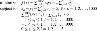 |
The problem consists of a quadratic objective function, 1,000 linear equality constraints, and a linear inequality constraint. There are also 2,005 variables. The goal is to find a local minimum by using the ACTIVESET technique. This can be accomplished by issuing the following call to PROC OPTMODEL:
proc optmodel;
   number n = 1000;
   number b = 5;
   var x{1..n} >= -1 <= 1 init  0.99;
   var y{1..n} >= -1 <= 1 init -0.99;
   var z{1..b} >=  0 <= 2 init  0.5;
   minimize f = sum {i in 1..n} x[i] * y[i] + sum {j in 1..b} 0.5 * z[j]^2;
   con cons1{k in 1..n}: x[k] + y[k] + sum {j in 1..b} z[j] = b;
   con cons2: sum {i in 1..n} (x[i] + y[i]) + sum {j in 1..b} z[j] >= b + 1;
   solve with NLP / tech=activeset printfreq=10;
quit;
The SAS output displays a detailed summary of the problem along with the status of the solver at termination, the total number of iterations required, and the value of the objective function at the local minimum. The summaries are shown in Figure 7.3.
| Problem Summary | |
|---|---|
| Objective Sense | Minimization |
| Objective Function | f |
| Objective Type | Quadratic |
| Number of Variables | 2005 |
| Bounded Above | 0 |
| Bounded Below | 0 |
| Bounded Below and Above | 2005 |
| Free | 0 |
| Fixed | 0 |
| Number of Constraints | 1001 |
| Linear LE (<=) | 0 |
| Linear EQ (=) | 1000 |
| Linear GE (>=) | 1 |
| Linear Range | 0 |
| Solution Summary | |
|---|---|
| Solver | NLP/ACTIVESET |
| Objective Function | f |
| Solution Status | Optimal |
| Objective Value | -996.5 |
| Iterations | 5 |
| Optimality Error | 2.5083794E-8 |
| Infeasibility | 7.0654349E-8 |
The SAS log shown in Figure 7.4 displays a brief summary of the problem that is being solved, followed by the iterations that are generated by the solver.
| NOTE: The problem has 2005 variables (0 free, 0 fixed). |
| NOTE: The problem has 1001 linear constraints (0 LE, 1000 EQ, 1 GE, 0 range). |
| NOTE: The problem has 9005 linear constraint coefficients. |
| NOTE: The problem has 0 nonlinear constraints (0 LE, 0 EQ, 0 GE, 0 range). |
| NOTE: The OPTMODEL presolver removed 0 variables, 0 linear constraints, and 0 |
| nonlinear constraints. |
| NOTE: Using analytic derivatives for objective. |
| NOTE: Using 2 threads for nonlinear evaluation. |
| NOTE: The NLP solver is called. |
| NOTE: The experimental Active Set algorithm is used. |
| Objective Optimality |
| Iter Value Infeasibility Error |
| 0 -979.47500000 3.50000000 0.50000000 |
| 10 -996.49999990 0.0000000006047 0.0000000023898 |
| NOTE: Optimal. |
| NOTE: Objective = -996.5. |
An Optimization Problem with Many Local Minima
Consider the following optimization problem:
 |
The objective function is highly nonlinear and contains many local minima. The NLP solver provides you with the option of searching the feasible region and identifying local minima of better quality. This is achieved by writing the following SAS program:
proc optmodel;
  var x >= -1 <= 1;
  var y >= -1 <= 1;
  min f = exp(sin(50*x)) + sin(60*exp(y)) + sin(70*sin(x)) + sin(sin(80*y))
          - sin(10*(x+y)) + (x^2+y^2)/4;
  solve with nlp / MULTISTART;
quit;
The MULTISTART option is specified, which directs the algorithm to start the local solver from many different starting points. The SAS log is shown in Figure 7.5.
| NOTE: The problem has 2 variables (0 free, 0 fixed). |
| NOTE: The problem has 0 linear constraints (0 LE, 0 EQ, 0 GE, 0 range). |
| NOTE: The problem has 0 nonlinear constraints (0 LE, 0 EQ, 0 GE, 0 range). |
| NOTE: The OPTMODEL presolver removed 0 variables, 0 linear constraints, and 0 |
| nonlinear constraints. |
| NOTE: Using analytic derivatives for objective. |
| NOTE: Using 2 threads for nonlinear evaluation. |
| NOTE: The NLP solver is called. |
| NOTE: The Interior Point algorithm is used. |
| NOTE: The experimental MULTISTART option is enabled. |
| Best Local Optimality Local |
| Start Objective Objective Infeasibility Error Status |
| 1 -1.3289 -1.3289 0 5e-07 OPT |
| 2 -2.2337 -2.2337 0 5e-07 OPT |
| 3 -2.4362 -2.4362 0 5e-07 OPT |
| 4 -2.9597 -2.9597 0 5e-07 OPT |
| 5 -2.9597 -0.15307 0 5e-07 OPT |
| 6 -2.9597 -0.78675 0 5e-07 OPT |
| 7 -3.2081 -3.2081 0 5e-07 OPT |
| 8 -3.2081 -0.6604 0 5e-07 OPT |
| 9 -3.2081 -2.7358 0 5e-07 OPT |
| 10 -3.2081 -1.3429 0 5e-07 OPT |
| 11 -3.2081 -1.8175 0 5e-07 OPT |
| 12 -3.2081 0.34388 0 5e-07 OPT |
| 13 -3.2081 -1.7222 0 5e-07 OPT |
| 14 -3.2081 0.78923 0 5e-08 OPT |
| 15 -3.2081 -1.3697 0 5e-07 OPT |
| 16 -3.2081 0.34917 0 5e-07 OPT |
| 17 -3.2081 -1.2485 0 5e-07 OPT |
| 18 -3.2081 -2.2667 0 5e-07 OPT |
| 19 -3.2081 -1.806 0 5e-07 OPT |
| 20 -3.2081 -1.4817 0 5e-07 OPT |
| 21 -3.2081 -2.3113 0 5e-07 OPT |
| 22 -3.2081 -2.3871 0 5e-07 OPT |
| 23 -3.2081 -1.247 0 5e-07 OPT |
| 24 -3.2081 0.21282 6.6372e-08 4.021e-06 BESTFEAS |
| 25 -3.2081 -2.9526 0 5e-07 OPT |
| 26 -3.2081 -2.8503 0 5e-07 OPT |
| 27 -3.2081 0.1177 0 5e-07 OPT |
| 28 -3.2081 -1.0823 0 5e-07 OPT |
| 29 -3.2081 -0.90374 0 1.7236e-05 BESTFEAS |
| 30 -3.2081 -1.5839 0 5e-07 OPT |
| 31 -3.2081 -2.1584 0 5e-07 OPT |
| 32 -3.2081 -0.61349 0 5e-07 OPT |
| 33 -3.2081 0.30541 0 5e-07 OPT |
| 34 -3.2081 -1.3731 0 5e-07 OPT |
| 35 -3.2081 -0.32353 0 5e-07 OPT |
| NOTE: Multistart used 35 starting points. |
| NOTE: Best optimal objective = -3.20813913. |
| NOTE: Best optimal solution is found at starting point 7. |
The SAS log presents additional information when the MULTISTART option is enabled. The first column counts the number of restarts of the local solver. The second column records the best local optimum that has been found so far, and the third column records the local optimum to which the solver has converged. The final column records the status of the local solver at every iteration.
The SAS output is shown in Figure 7.6.
| Problem Summary | |
|---|---|
| Objective Sense | Minimization |
| Objective Function | f |
| Objective Type | Nonlinear |
| Number of Variables | 2 |
| Bounded Above | 0 |
| Bounded Below | 0 |
| Bounded Below and Above | 2 |
| Free | 0 |
| Fixed | 0 |
| Number of Constraints | 0 |
| Solution Summary | |
|---|---|
| Solver | NLP/INTERIORPOINT |
| Objective Function | f |
| Solution Status | Optimal |
| Objective Value | -3.20813913 |
| Iterations | 35 |
| Optimality Error | 5E-7 |
| Infeasibility | 0 |