| The NLP Procedure |
Example 4.6: Maximum Likelihood Weibull Estimation
Two-Parameter Weibull Estimation
The following data are taken from Lawless (1982, p. 193) and represent the number of days it took rats painted with a carcinogen to develop carcinoma. The last two observations are censored data from a group of 19 rats:
    data pike;
       input days cens @@;
       datalines;
    143  0  164  0  188  0  188  0
    190  0  192  0  206  0  209  0
    213  0  216  0  220  0  227  0
    230  0  234  0  246  0  265  0
    304  0  216  1  244  1
    ;
Suppose that you want to show how to compute the maximum likelihood estimates
of the scale parameter ![]() (
(![]() in Lawless), the shape
parameter
in Lawless), the shape
parameter ![]() (
(![]() in Lawless), and the location parameter
in Lawless), and the location parameter
![]() (
(![]() in Lawless). The observed likelihood function of
the three-parameter Weibull transformation (Lawless 1982, p. 191) is
in Lawless). The observed likelihood function of
the three-parameter Weibull transformation (Lawless 1982, p. 191) is
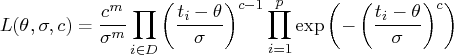
and the log likelihood is

The log likelihood function can be evaluated only for
![]() ,
, ![]() , and
, and ![]() . In the
estimation process, you must enforce these conditions using
lower and upper boundary constraints.
The three-parameter Weibull estimation can be numerically
difficult, and it usually pays off to provide good initial
estimates. Therefore, you first estimate
. In the
estimation process, you must enforce these conditions using
lower and upper boundary constraints.
The three-parameter Weibull estimation can be numerically
difficult, and it usually pays off to provide good initial
estimates. Therefore, you first estimate ![]() and
and ![]() of
the two-parameter Weibull distribution for constant
of
the two-parameter Weibull distribution for constant ![]() .
You then use the optimal parameters
.
You then use the optimal parameters ![]() and
and ![]() as starting values for the three-parameter Weibull estimation.
as starting values for the three-parameter Weibull estimation.
Although the use of an INEST= data set is not really necessary for this simple example, it illustrates how it is used to specify starting values and lower boundary constraints:
    data par1(type=est);
       keep _type_ sig c theta;
       _type_='parms'; sig = .5;
          c = .5; theta = 0; output;
       _type_='lb'; sig = 1.0e-6;
          c = 1.0e-6; theta = .;  output;
    run;
The following PROC NLP call specifies the maximization of the
log likelihood function for the two-parameter Weibull estimation
for constant ![]() :
:
    proc nlp data=pike tech=tr inest=par1 outest=opar1
         outmodel=model cov=2 vardef=n pcov phes;
       max logf;
       parms sig c;
       profile sig c / alpha = .9 to .1 by -.1 .09 to .01 by -.01;

       x_th = days - theta;
       s    = - (x_th / sig)**c;
       if cens=0 then s + log(c) - c*log(sig) + (c-1)*log(x_th);
       logf = s;
    run;
After a few iterations you obtain the solution given in Output 4.6.1.
Output 4.6.1: Optimization ResultsSince the gradient has only small elements and the Hessian (shown in Output 4.6.2) is negative definite (has only negative eigenvalues), the solution defines an isolated maximum point.
Output 4.6.2: Hessian Matrix atThe square roots of the diagonal elements of the approximate covariance matrix of parameter estimates are the approximate standard errors (ASE's). The covariance matrix is given in Output 4.6.3.
Output 4.6.3: Covariance MatrixThe confidence limits in Output 4.6.4 correspond to the ![]() values
in the PROFILE statement.
values
in the PROFILE statement.
| ||||||||||||||||||||||||||||||||||||||||||||||||||||||||||||||||||||||||||||||||||||||||||||||||||||||||||||||||||||||||||||||||||||||||||||||||||||||||||||||||||||||||||||||||||||||||||||||||||||||||||||||||||||||||||||||||||||||||||||||||||||||||||||||||||||||||||||||||||||||||||||||||||||||||||||||||
Three-Parameter Weibull Estimation
You now prepare for the three-parameter Weibull estimation by using PROC UNIVARIATE to obtain the smallest data value for the upper boundary constraint for
    /* Calculate upper bound for theta parameter */
    proc univariate data=pike noprint;
       var days;
       output out=stats n=nobs min=minx range=range;
    run;
    data stats;
       set stats;
       keep _type_ theta;

       /* 1. write parms observation */
       theta = minx - .1 * range;
       if theta < 0 then theta = 0;
       _type_ = 'parms';
       output;

       /* 2. write ub observation */
       theta = minx * (1 - 1e-4);
       _type_ = 'ub';
       output;
    run;
The data set PAR2 specifies the starting values and the lower and upper bounds for the three-parameter Weibull problem:
    proc sort data=opar1;
       by _type_;
    run;

    data par2(type=est);
       merge opar1(drop=theta) stats;
       by _type_;
       keep _type_ sig c theta;
       if _type_ in ('parms' 'lowerbd' 'ub');
    run;
The following PROC NLP call uses the MODEL= input data set containing the log likelihood function that was saved during the two-parameter Weibull estimation:
    proc nlp data=pike tech=tr inest=par2 outest=opar2
          model=model cov=2 vardef=n pcov phes;
       max logf;
       parms sig c theta;
       profile sig c theta / alpha = .5 .1 .05 .01;
    run;
After a few iterations, you obtain the solution given in Output 4.6.5.
Output 4.6.5: Optimization ResultsPROC NLP: Nonlinear Maximization
Value of Objective Function = -87.32424712
| ||||||||||||||||||||||||||||||||||||||||||
From inspecting the first- and second-order derivatives at the optimal solution, you can verify that you have obtained an isolated maximum point. The Hessian matrix is shown in Output 4.6.6.
Output 4.6.6: Hessian MatrixThe square roots of the diagonal elements of the approximate covariance matrix of parameter estimates are the approximate standard errors. The covariance matrix is given in Output 4.6.7.
Output 4.6.7: Covariance MatrixThe difference between the Wald and profile CLs for parameter PHI2 are remarkable, especially for the upper 95% and 99% limits, as shown in Output 4.6.8.
Output 4.6.8: Confidence Limits
| ||||||||||||||||||||||||||||||||||||||||||||||||||||||||||||||||||||||||||||||||||||||||||||||||||||||||||||||||
Copyright © 2008 by SAS Institute Inc., Cary, NC, USA. All rights reserved.