IMSTAT Procedure (Analytics)
- Syntax
 Procedure SyntaxPROC IMSTAT (Analytics) StatementAGGREGATE StatementARM StatementASSESS StatementBOXPLOT StatementCLUSTER StatementCORR StatementCROSSTAB StatementDECISIONTREE StatementDISTINCT StatementFORECAST StatementFREQUENCY StatementGENMODEL StatementGLM StatementGROUPBY StatementHISTOGRAM StatementHYPERGROUP StatementKDE StatementLOGISTIC StatementMDSUMMARY StatementNEURAL StatementOPTIMIZE StatementPERCENTILE StatementRANDOMWOODS StatementREGCORR StatementSUMMARY StatementTEXTPARSE StatementTOPK StatementTRANSFORM StatementQUIT Statement
 - Overview
- Using
- Examples Calculating Percentiles and QuartilesRetrieving Box ValuesRetrieving Box Plot Values with the NOUTLIERLIMIT= OptionRetrieving Distinct Value Counts and GroupingPerforming a Cluster AnalysisPerforming a Pairwise CorrelationCrosstabulation with Measures of Association and Chi-Square TestsTraining and Validating a Decision TreeStoring and Scoring a Decision TreePerforming a Multi-Dimensional SummaryFitting a Regression ModelForecasting and Automatic ModelingForecasting with Goal SeekingAggregating Time Series DataTraining and Validating a Neural NetworkPredicting Email Spam and Assessing the ModelTransforming Variables with Imputation and Binning
GLM Statement
The GLM statement is used to fit models that are similar to those handled by the GLM procedure. There are some important differences in syntax and functionality between the GLM procedure and the GLM statement in IMSTAT.
Syntax
Required Arguments
dependent-variable
specifies the variable to model. This variable is also referred to as the response variable.
model-effects
specifies a list of variables to use for modeling the dependent variable.
Optional Argument
class-variables
specifies a list of variables to use as classification variables. The variables in this list take the place of the CLASS statement in traditional SAS procedures.
GLM Statement Options
ALLIDVARS
requests that all variables in the input table are treated as ID variables when a scoring table is produced. In other words, if this option is specified, all variables from the input table, including computed columns, are transferred to the scoring table. This option has no effect unless you specify the SCORE option.
ALPHA=number
specifies a number between 0 and 1 from which to determine the confidence level for approximate confidence intervals of the parameter estimates. The default is α = 0.05, which leads to 100 x (1- α)% = 95% confidence limits for the parameter estimates.
| Default | 0.05 |
CHISQ
requests that p-values in the table of parameter estimates and Type III tests are determined as probabilities under a x2 distribution. This means that instead of two-sided p-values based on the t distribution, the p-values are computed as two-sided probabilities under a standard normal distribution. Similarly, the assumption of F distributions with finite denominator degrees of freedom is ignored in lieu of assuming infinite degrees of freedom.
CI
specifies to add confidence intervals to the table of parameter estimates. The confidence level is 100*(1-α)% where α is determined by the ALPHA= option. The default value is α = 0.05. This value is equivalent to a 95% confidence limit.
| Default | 0.05 |
CLASSFORMATS=("format-name1"<, "format-name2" ...>)
specifies the formats for the classification variables in the model. If you do not specify the CLASSFORMATS= option, the default format is applied for the classification variable. That default format was determined when the table was originally loaded into the server. In the following example, the CLASSFORMAT= values apply to variables x1 and x2.
| Alias | CLASSFMT= |
| Example | glm y (x1 x2) = x3-x7 / classformats=("YN.", "F8."); |
CODE <(code-generation-options)>
requests that the server produce SAS scoring code based on the actions that it performed during the analysis. The server generates DATA step code. By default, the code is replayed as an ODS table by the procedure as part of the output of the statement. More frequently, you might want to write the scoring code to an external file by specifying options.
Y, the
generated code stores the predicted value as P_Y.
The name of the variable is truncated to fit within the SAS name length
requirements.
COMMENT
specifies to add comments to the code in addition to the header block. The header block is added by default.
FILENAME='path'
specifies the name of the external file to which the scoring code is written. This suboption applies only to the scoring code itself. If you request that the server generate IMSTAT programming statements with the IMSTAT suboption, then these statements are saved as an ODS table.
| Alias | FILE= |
FORMATWIDTH=k
specifies the width to use in formatting derived numbers such as parameter estimates in the scoring code. The server applies the BEST format, and the default format for code generation is BEST20.
| Alias | FMTW= |
| Range | 4 to 32 |
IMSTAT
specifies to generate IMSTAT programming statements that reproduce the analysis in addition to the scoring code. For example, this option is helpful when you perform variable selection and you want to capture the modeling code that reflects only the selected variables.
IMSTATONLY
specifies to generate the IMSTAT programming statements only. No scoring code is produced.
LABELID=id
specifies a group identifier for group processing. The identifier is an integer and is used to create array names and statement labels in the generated code.
LINESIZE=n
specifies the line size for the generated code.
| Alias | LS= |
| Default | 72 |
| Range | 64 to 256 |
NOTRIM
requests that the comparison of the formatted values for class variables and group-by variables is based on the full format width with padding. By default, the leading and trailing blanks are removed from the formatted values.
REPLACE
specifies to overwrite the external file with the new contents if the file already exists. This option has no effect unless you specify the FILENAME= option.
EXCLUDE=(list-of-ODS-tables)
specifies the result tables that you want to exclude from being generated on the server and from being sent to the SAS session. The GLM statement can generate the following tables:
|
Table Name
|
Table Alias
|
Description
|
Condition
|
|---|---|---|---|
|
ModelInfo
|
Information about the
model—constant across groups or partitions.
|
This table is shown
by default.
|
|
|
ClassLevels
|
Class
|
Information about the
classification variables, such as the number of levels and their values.
|
This table is shown
when classification variables are present in the model.
|
|
Dimensions
|
Dim
|
Model dimensions
|
This table is shown
by default.
|
|
FitStatistics
|
Fit
|
Fit statistics customary
for generalized linear models
|
This table is shown
when it is requested with the SELECT= option.
|
|
OverallAnova
|
GlobalAnova
|
Model, source, and error
decomposition of variation
|
This table is shown
when classification variables are present in the model.
|
|
ModelAnova
|
ANOVA
|
Variance decomposition
with significance tests for all model effects
|
This table is shown
when classification variables are present in the model.
|
|
ParameterEstimates
|
ParmEstimates
Pest
|
The solutions for the
linear model coefficients
|
This table is shown
when there are no classification variables in the model.
|
|
Tests3
|
Type III tests of model
effects
|
This table is shown
when it is requested with the SELECT= option.
|
FORMATS=("format-specification"<,...>)
specifies the formats for the GROUPBY variables. If you do not specify the FORMATS= option, or if you omit the entry for a GROUPBY variable, the default format is applied for that variable.
| Example | proc imstat data=lasr1.table1; statement / groupby=(a b) formats=("8.3", "$10"); quit; |
FREQ=variable-name
specifies the numeric variable that provides frequencies for the analysis. For example, if the FREQ= variable has the value 5, then it implies that the record represents five such observations with identical values for the modeling variables. If you specify a FREQ= variable, then only the observations with a value that is not missing and greater than zero for the variable are used in the analysis.
GROUPBY=(variable-list)
specifies a list of variable names, or a single variable name, to use as GROUPBY variables in the order of the grouping hierarchy. If you do not specify any GROUPBY variable names, then the calculation is performed across the entire table—possibly subject to a WHERE clause.
GROUPBYMODE= DATA | MODEL | LASR
specifies the parallelization technique for group-by processing. The default is GROUPBYMODE=MODEL in which threads solve separate models following a lateral reconciliation of cross-product matrices. This mode is appropriate in situations with many groups and relatively small cross-product matrices. Model-parallel processing minimizes passes through the data.
| Default | MODEL |
GROUPFILTER=(filter-options)
specifies a section of the group-by hierarchy to be included in the computation. With this option, you can request that the server performs the analysis for only a subset of all possible groupings. The subset is determined by applying the group filter to a temporary table that you generate with the GROUPBY statement.
DESCENDING
specifies the top section or the bottom section of the groupings to be collected. If the DESCENDING option is specified, the top LIMIT=n (where n > 0) groupings are collected. Otherwise, the bottom LIMIT=n groupings are collected.
| Alias | DESC |
LIMIT=n
specifies the maximum number of distinct groupings to be collected, where integer n >= 0. If n is zero, then all distinct groupings (up to 231–1) that satisfy the boundary constraints, such as LOWERSCORE=f, are collected.
| CAUTION: |
High Cardinality
Data Sets
Setting n to
zero with high-cardinality data sets can significantly delay the response
of the server.
|
SCOREGT=f
specifies the exclusive lower bound for the numeric scores of the distinct groupings to collect.
| Alias | SGT= |
SCORELT=f
specifies the exclusive upper bound for the numeric scores of the distinct groupings to collect.
| Alias | SLT= |
VALUEGT=("format-name1" <, "format-name2" ...>)
specifies the exclusive lower bound of the group-by variable’s formatted values for the distinct groupings to collect.
| Alias | VGT= |
VALUELT=("format-name1" <, "format-name2" ...>)
specifies the exclusive upper bound of the group-by variable’s formatted values for the distinct groupings to collect.
| Alias | VLT= |
TABLE=table-with-groupby-results
specifies the in-memory table from which to load the group-by hierarchy. If the TABLE= option is not specified, then all other GROUPFILTER= options are ignored.
proc imstat;
    table example.cars_program_all;
    groupby state city trade_in_model / temptable
                 weight=new_vehicle_msrp
                 agg   =(max)
                 order =weight;
run; table example.cars_program_all;
distinct sales_type / groupfilter=(
table =mylasr.&_TEMPLAST_
scoregt=40000
valuelt=("FL","Ft Myers","")
limit =20
descending);
run;| Interaction | If you specify the GROUPFILTER= option, then the GROUPBY= and FORMATS= options have no effect. |
IDVARS=(variable-list)
IDVARS=variable-name
specifies the variables from the active table to transfer to the temporary table that is created by scoring the input table. This option has no effect unless the SCORE option is also specified. (See the SCORE option for details about which variables are added to the temporary table by default.) The IDVARS= option should be used to transfer additional columns from the input table to the scoring table.
| Alias | ID= |
| Tip | Instead of this option, you can specify the ALLIDVARS option to transfer all variables from the input table to the scoring table. |
INCLUDEMISS
specifies to treat missing values for classification variables as valid levels. If the INCLUDEMISS option is not specified, observations with missing values in the classification variables are not used in the analysis.
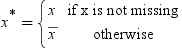
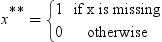
INFORMATIVE
requests that missing values are handled by modeling them through extra model effects. These effects consist of dummy variables that take on the value 1 when the value of a continuous model variable that is involved in the effect is missing. Otherwise, they are assigned the value 0. The missing value in the original model effect is replaced with the average value for the effect for the nonmissing values.
| Alias | INFORMMISS |
KEYORDER
requests that the results for a partitioned analysis are displayed in the order of the partition keys. If this option is not specified, then results are displayed by using the partitions on the first worker node followed by the partitions on the second node, and so on. Without this option, the results are likely to have random ordering of the partitions. The KEYORDER option makes result collection less efficient but produces a natural, predictable order.
MAXTESTLEV=n
specifies the maximum number of levels in an effect for which the server generates Type III tests. The idea behind the MAXTESTLEV= option is that testing effects for significance that have a large number of levels is typically not meaningful. The effects tend to be highly significant anyway, but determining the exact significance level is computationally intensive. The default value is 300 and implies that no test statistics are produced for any effect that has more than 300 levels.
| Default | 300 |
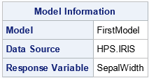
NAME=SAS-name
specifies the name to use for identifying the model in the server output and in the temporary table of results generated by the TEMPTABLE option. SAS name rules apply. For example, the following statements add the 'Model' entry to the ModelInformation table.
proc imstat;
   table hps.iris;
   glm sepalwidth = sepallength / name = FirstModel;
run;
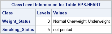
NOCLPRINT <=n>
specifies the number of levels for each classification variables to show in the Class Level Information ODS table. If you do not specify the NOCLPRINT option, all unique values are shown in the order of the class variable levelization. If you specify NOCLPRINT=n, then the values are shown for those classification variables that have less than n levels only. The value for n must be at least 1.
NOINT
suppresses the inclusion of an intercept in the model. By default, the GLM statement adds an intercept as the first model effect to the model. Exclusion of the intercept is useful in certain models to achieve a desired interpretation of the model effects.
glm y (A) = A / noint;
NOPREPARSE
prevents the procedure from preparsing and pregenerating code for temporary expressions, scoring programs, and other user-written SAS statements.
| Alias | NOPREP |
PARTITION<=partition-key>
specifies to fit the model separately for each value of the partition key. In other words, the partition variables function as automatic group-by variables for the request.
| Alias | PART= |
ROLEVAR=variable-name
specifies a variable in the in-memory table that defines whether an observation belongs to the training set, the validation set, or is to be excluded from the analysis. The role variable can have a numeric or character type, and it can be a temporary computed variable.
-
value = 1: this observation is in the training set
-
value = 2: this observation is in the validation set
-
any other value: this observation is to be excluded from the analysis
-
If the first non-blank character is 't' or 'T', then the observation is in the training set.
-
If the first non-blank character is 'v' or 'V', then he observation is in the validation set.
-
Any other value for the first non-blank character, including an all blank entry, leads to the exclusion of the observation from the analysis.
| Alias | ROLE= |
| Interactions | You can divide the data at random into training and validation sets by providing the VALIDATE= and SEED= options. |
| If you specify both the ROLEVAR= option and the VALIDATE= options, then the ROLEVAR= setting supersedes the VALIDATE= option. |
SCORE <(score-statistic1 score-statistic2 ...)>
requests that the active table be scored after the model is fit and the results be stored in a temporary table. The server automatically adds all model variables to the temporary table with the score results. These results include the response variable, the class variables, all explanatory variables from which effects are formed, and the WEIGHT=, and FREQ= variables.
|
Keyword and Aliases
|
Column Name
|
Description
|
Default
|
|---|---|---|---|
|
PRED, PREDICTED, MEAN
|
_PRED_
|
Predicted value
|
Yes
|
|
RESID, RESIDUAL, R
|
_RESID_
|
Raw residual (observed
- predicted)
|
Yes
|
|
STUDENT
|
_STUDENT_
|
Studentized residual
|
Yes
|
|
RSTUDENT
|
_RSTUDENT_
|
Studentized residual
with the current observation removed
|
Yes
|
|
LEVERAGE, H
|
_LEVERAGE_
|
Leverage value of the
observation
|
Yes
|
|
STDP
|
_STDP_
|
Standard error of the
mean predicted value
|
No
|
|
STDR
|
_STDR_
|
Standard error of the
residual
|
No
|
|
STDI
|
_STDI_
|
Standard error of the
(individual) predicted value
|
No
|
|
LCLM, LOWERMEAN
|
_LCLM_
|
Lower confidence limit
for the mean of the predicted value
|
No
|
|
UCLM, UPPERMEAN
|
_UCLM_
|
Upper confidence limit
for the mean of the predicted value
|
No
|
|
LCL, LOWERPRED
|
_LCL_
|
Lower confidence limit
for the predicted value
|
No
|
|
UCL, UPPERPRED
|
_UCL_
|
Upper confidence limit
for the predicted value
|
No
|
|
COOKD, COOKSD
|
_COOKD_
|
Cook's D influence
measure
|
No
|
|
DFFITS
|
_DFFITS_
|
Standardized influence
of the observation on predicted value
|
No
|
|
COVRATIO
|
_COVRATIO_
|
Standardized influence
of the observation on the covariance matrix of the parameter estimates
|
No
|
|
LIKEDIST, LD
|
_LIKEDIST_
|
Displacement (distance)
of log-likelihood when the observation is removed (assuming normal
distribution)
|
No
|
SEED=number
specifies the random number seed for generating random numbers. The random number is used to determine whether an observation belongs to the training or validation data set. The SEED= option has no effect unless you specify the VALPROP= option. If the specified number is negative or zero, the random number generation is based on the computer clock of the server—this generates a non-reproducible random number sequence.
SELECT=(list-of-ODS-tables)
specifies the list of ODS tables that you want to display for the analysis. The specified list replaces the default tables that are generated by the server and displayed. See the EXCLUDE= option for the list of default tables and the table names that you can display.
SHOWSELECTED
requests that the server perform variable selection for the model. A backward selection method is used, where the significance level for an effect to remain in the model is determined by the SLSTAY= option. This option performs variable selection like the VARSEL option, but in contrast to the latter option, it displays output only for the selected effects.
| Alias | SHOWSEL |
SLSTAY=α
specifies the significance level used in determining whether effects should stay in the model during variable selection.
| Default | 0.1 |
| Range | 0 to 1 |
TEMPEXPRESS="SAS-expressions"
TEMPEXPRESS=file-reference
specifies either a quoted string that contains the SAS expression that defines the temporary variables or a file reference to an external file with the SAS statements.
| Alias | TE= |
TEMPNAMES=variable-name
TEMPNAMES=(variable-list)
specifies the list of temporary variables for the request. Each temporary variable must be defined through SAS statements that you supply with the TEMPEXPRESS= option.
| Alias | TN= |
TEMPTABLE
generates an in-memory temporary table from the result set. The IMSTAT procedure displays the name of the table and stores it in the macro variable, provided that the statement executed successfully.
| Interaction | For information about the interaction between the TEMPTABLE, CODE, and SCORE options, see Temporary Tables, Generated Code, and Scoring. |
VALIDATE=f
specifies the proportion f in the validation data set.
| Alias | VALPROP= |
| Range | 0 to 1 |
| Interaction | If you specify both the ROLEVAR= option and the VALIDATE= option, then the ROLEVAR= setting supersedes the VALIDATE= option. |
VARSELECTION
specifies that the server perform variable selection for the model. A backward selection method is used, where the significance level for an effect to remain in the model is determined by the SLSTAY= option. In contrast to the SHOWSEL option, all effects are reported in the IMSTAT output.
| Alias | VARSEL |
VIF
produces variance inflation factors and tolerances, the reciprocal of the VIF, for the parameter estimates.
WEIGHT=variable-name
specifies the numeric variable to use as a weighing variable in solving the linear model.

Details
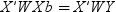
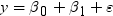
Basic Syntax

-
to estimate the unknowns β and σ2
-
to diagnose the appropriateness of the specified model
-
to select appropriate variables and terms for the X matrix
-
to predict the average response and unobserved values of the response variable with confidence
-
to test hypotheses about the elements of β provided that the model is acceptable
-
the intercept is included by default in every model. It is then the leading effect in X and simply adds a column of ones to this matrix. The intercept can be approximately interpreted as an adjustment for the mean of the response variable.
-
a continuous effect consists of only numeric non-class variables. The simplest continuous effect contains only one variable. For example, if you add the numeric variable Age to the model, you are adding a continuous effect. If the variable Height is not a classification variable, and you add the term Age*Height to the model, you are adding a continuous interaction effect.
-
a classification variable is a variable that is used in the model not through its raw values, but through an encoding of its unique (formatted) values. For example, if variable Gender is used as a classification variable in the model, then it represents two levels.
-
a classification effect is a model effect that contains one or more classification variables. A "pure" classification effect comprises only classification variables, a continuous classification effect also involves some continuous variables.
-
If A and B are classification variables, and X and Z are non-classification variables, then the effects A, B, and A*B are pure classification effects, termed the A and B main effect and the interaction of A and B, respectively. The effect A*Z would be a continuous classification effect.
-
Effect A is said to be nested within effect B if levels of A within one level of B do not mean the same thing for other levels of B. Nested effects are expressed with parenthetical notation. For example, if City and State are classification variables, then City(State) represents the nested effect of cities within states. One example of appropriate nesting is when city #1 in Alaska refers to a different city than city #1 in Colorado.
-
Two effects are said to be crossed if the levels of one effect retain their interpretation across the levels of the other effect. If Married is a classification variable that groups individuals into married and unmarried status, and Gender is a two-level variable, the Gender*Married effect is crossed, because a man in the unmarried group is also a man in the married group.
-
-
A character variable that is used in a model effect is treated as a classification variable.
-
A numerical variable that is used in a model effect is treated as a non-classification variable.
-
All variables explicitly listed in the optional variable list that follows the specification of the dependent variable in the GLM statement are classification variables.
-
The role of temporary computed variables is determined by the data type.
-
If the computed column is of character type, then it is automatically added to the model as a classification variable if it appears in a model effect.
-
If the computed column is of numeric type, then it is treated as a classification variable only if it is specified in the list of class-variables.
-
glm height = weight sex;
glm height(sex) = weight sex;
table lasr.class(tempnames=(t1 t2));
glm height = t1 t2 / tn=(t1 t2) te="t1=weight; t2=sex;";
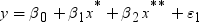
Informative Missingness
 . Because the estimate for the intercept is
  in the simple linear regression model, the predicted
value would be the average response of the nonmissing values,
in the simple linear regression model, the predicted
value would be the average response of the nonmissing values,  .
.
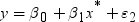
 for the missing values during training. This can
be seen, since the model that simply substitutes for the missing values is as follows:
for the missing values during training. This can
be seen, since the model that simply substitutes for the missing values is as follows:
 measures the amount by which the predicted value
differs from a predicted value at .
measures the amount by which the predicted value
differs from a predicted value at .