IMSTAT Procedure (Analytics)
- Syntax
 Procedure SyntaxPROC IMSTAT (Analytics) StatementAGGREGATE StatementARM StatementASSESS StatementBOXPLOT StatementCLUSTER StatementCORR StatementCROSSTAB StatementDECISIONTREE StatementDISTINCT StatementFORECAST StatementFREQUENCY StatementGENMODEL StatementGLM StatementGROUPBY StatementHISTOGRAM StatementHYPERGROUP StatementKDE StatementLOGISTIC StatementMDSUMMARY StatementNEURAL StatementOPTIMIZE StatementPERCENTILE StatementRANDOMWOODS StatementREGCORR StatementSUMMARY StatementTEXTPARSE StatementTOPK StatementTRANSFORM StatementQUIT Statement
 - Overview
- Using
- Examples Calculating Percentiles and QuartilesRetrieving Box ValuesRetrieving Box Plot Values with the NOUTLIERLIMIT= OptionRetrieving Distinct Value Counts and GroupingPerforming a Cluster AnalysisPerforming a Pairwise CorrelationCrosstabulation with Measures of Association and Chi-Square TestsTraining and Validating a Decision TreeStoring and Scoring a Decision TreePerforming a Multi-Dimensional SummaryFitting a Regression ModelForecasting and Automatic ModelingForecasting with Goal SeekingAggregating Time Series DataTraining and Validating a Neural NetworkPredicting Email Spam and Assessing the ModelTransforming Variables with Imputation and Binning
HYPERGROUP Statement
The HYPERGROUP statement analyzes a graph whose vertices are identified by values of the analysis variables and whose edges are named by those variables within the same observation. The analysis that can be performed falls into three general areas: structural analysis of the overall graph, centrality calculation for individual vertices, and layout of the graph in either 2-D or 3-D space.
Syntax
Optional Argument
variable-list
specifies the variables to include in the analysis. The variables must have a character data type. Separate variable names with a space. If you do not specify any variables, then all character variables in the active table are used in the analysis.
HYPERGROUP Statement Options
C=relative-strength
specifies the relative strength of local forces to global forces with regard to laying out the positions of vertices and edges. The Walshaw layout is a force-directed algorithm that finds positions of vertices so that no vertices are too close together and so that (usually) edges are about the same length. The force term in a force-directed layout algorithm is related to springs. Imagine each vertex is a ring and each edge is a spring whose ends are hooked around the rings of the vertices to which the edge connects.
| Default | 0.01 |
| Applies to | LAYOUT=WALSHAW |
CENTRALITY
specifies to quantify the importance of each vertex among its peers. Many types of centrality have been defined. The HYPERGROUP statement supports five that are commonly used. Four of these are based on shortest paths (the smallest number of edges in a path from one vertex to the other). The fifth is a geometric measure that can be calculated when graph layout is performed. For more information, see Centrality Measures.
CLOSITERS=n
specifies the number of layout iterations that are performed before a sub-algorithm determines the vertices that are close to each other. Increasing the value can improve performance because more iterations are performed between attempts to evaluate which nodes are too close together.
| Default | 3 |
COMMALGORITHM= ASYNCHRONOUS |
COMMALGORITHM= SYNCHRONOUS | SEMISYNCHRONOUS
COMMALGORITHM= LLSYNCHRONOUS | LLSEMISYNCHRONOUS
specifies a particular label propagation algorithm when STRUCTURAL=COMMUNITY analysis is specified. The LL prefix indicates to use a parallel version of the algorithm.
| Alias | COMMALG |
COMMITERS=n
specifies the number of iterations to perform while determining communities. Communities are determined by a variant of the label propagation algorithm described in Raghavan, Reka, and Kumara (2007). The algorithm is iterative, and stops when COMMITERS= iterations have been performed.
| Default | 20 |
| Tip | The synchronous algorithms that are available with the COMMALG= option can require larger values for COMMITERS= for convergence to occur. |
COMMLAYOUTS
specifies to lay out coordinates for the community graph that is produced with the STRUCTURE=COMMUNITY (or BOTH) option. The coordinates shown are returned in the _TEMPHYPGRP3_ and TEMPEDGES3_ tables.
COMMMAX=n
specifies the maximum number of iterations to perform to determine labeling for communities. For the label propagation algorithm used when you specify STRUCTURAL=COMMUNITY, this option, together with COMMPRECENDENCE, alters tie-breaking schemes when there is a choice as to what value should be assigned to a vertex label.
COMMPRECEDENCE
An option for tuning the label propagation algorithm used with STRUCTUAL=COMMUNITIES analysis. See the explanation of the COMMMAX= option for details.
| Alias | COMMPRE |
CREATETEMPLAST= NEVER | ALWAYS | MULTIPLE
specifies when to create the _TEMPLAST_ temporary table that identifies the hypergroups and analysis variables. If you use a large active table with the HYPERGROUP statement, then the _TEMPLAST_ temporary table can be large as well.
NEVER
specifies to never create the _TEMPLAST_ temporary table. Be aware that the other in-memory temporary tables like _TEMPHYPGRP_ and _TEMPEDGES_ are created. These have summarized information about the hypergroups and are smaller than the _TEMPLAST_ table.
ALWAYS
specifies to create the _TEMPLAST_ temporary table.
MULTIPLE
specifies to create the _TEMPLAST_ temporary table when the analysis results in more than one hypergroup.
| Default | ALWAYS |
FAR_AWAY=d
specifies how to tune the layouts when LAYOUY=WALSHAW is specified.
| Default | 1 |
FORMATS=("format-specification",...)
specifies the formats for the GROUPBY= variables. If you do not specify the FORMAT= option, or if you do not specify the GROUPBY= option, the default format is applied for that variable.
GRAPHPARTITION
specifies to tune the layout to improve the separation of vertices. This option can increase the processing duration.
| Applies to | LAYOUT=WALSHAW or LAYOUT=FRUCHGOLD |
GROUPBY=(variable-list)
specifies a list of variable names, or a single variable name, to use as GROUPBY variables in the order of the grouping hierarchy. If you do not specify any GROUPBY variable names, then the calculation is performed across the entire table—possibly subject to a WHERE clause.
GROUPBYLIMIT=n
specifies the maximum number of levels in a GROUPBY set. When the software determines that there are at least n levels in the GROUPBY set, it abandons the action, returns a message, and does not produce a result set. You can specify the GROUPBYLIMIT= option if you want to avoid creating excessively large result sets in GROUPBY operations.
GROUPFILTER=(groupfilter-options)
specifies a section of the GROUPBY= hierarchy to include in the HYPERGROUP computation.
HEIGHT=z
specifies the maximum value for the frame's coordinate space in the Z-axis.
| Default | 100 units |
| Interaction | This option is used only when you specify the THREED option. |
HIGHDEGREE= 0 | 1
specifies to enable a heuristic that begins partitioning by eliminating vertices of unusually high degree. Some graphs have many vertices with low degree. The degree of a vertex is the number of edges that originate from or are directed toward the vertex. However, some graphs might have some vertices with very high degree. It is often beneficial to treat these high degree vertices as partitions early in the partitioning algorithm, even if they do not strictly split a graph. This simplifies the processing so that from what is left of the remaining graphs are less dense and faster to process.
| Default | 0 (disabled) |
| Range | 0 or 1 |
LAYOUT= WALSHAW | FRUCHGOLD | OTHER
specifies one of three force-directed algorithms to use for graph layout.
| Default | LAYOUT=WALSHAW |
LENGTH=y
specifies the maximum value for the frame's coordinate space in the Y-axis.
| Default | 100 units |
MARGIN=n
specifies the size of the border around the frame's coordinate space to remain free of vertices. For example, if you specify LENGTH=100, WIDTH=100, and MARGIN=12, then the frame coordinate space is 100 × 100 units and vertices have coordinates within the corners (12, 12), (12, 88), (88, 12), and (88, 88).
MAXNODES=n
specifies to tune graph partitioning by specifying the maximum number of nodes to permit in a partition. Each time a partitioning is performed, the resulting set of partitioned subgraphs is examined. If any exceed the maximum number of nodes specified in this option, then the partitioning is repeated on those partitions.
| Default | 4 |
MAXNVALS=i
specifies a positive integer that determines the maximum number of iterations for the percentile algorithm.
| Default | 1000 |
NITERATIONS=i
specifies a positive integer that determines the maximum number of iterations to execute for the forced-directed layout algorithm. A value between 200 and 5000 produces good results with most data sets. The LAYOUT=WALSHAW layout algorithm might stop before completing all NITER= iterations if the algorithm detects that convergence has occurred.
| Alias | NITERS |
| Default | 1000 |
NOCOLOR
specifies not to run the graph partitioning algorithm to assign colors to strongly connected communities. The algorithm is run by default. This option is useful if you do not use the color values. You can avoid the processing that is performed to assign color categories.
| Alias | NOCOLOUR |
NOCOORD
specifies not to perform graph layout of vertices and edges. Graph layout is the most time-consuming calculation that the HYPERGROUP statement performs. This option is useful if you do not need a visual or geometric layout, or calculation of centroid centrality. This option can improve the response time and conserve machine resources.
NOPENDANTS
specifies to simplify the graph layout by removing pendants (nodes of degree one). This option is performed repeatedly until no pendants remain in the graph.
NOVARS
specifies not to transfer additional variables to the _TEMPLAST_ table. See also VARS=.
PARTITION <=partition-key>
When you specify this option and the table is partitioned, the results are calculated separately for each value of the partition key. In other words, the partition variables function as automatic GROUPBY variables. This mode of executing calculations by partition is more efficient than using the GROUPBY= option. With a partitioned table, the server takes advantage of knowing that observations for a partition cannot be located on more than one worker node.
statement / partition="F          11"; /* passed directly to the server */
statement / partition="F","11";        /* composed by the procedure */
| Alias | PART= |
RADIANS
specifies to return the centroid centrality angles in radians rather than degrees.
| Applies to | CENTRALITY option |
SAVE=table-name
saves the result table so that you can use it in other IMSTAT procedure statements like STORE, REPLAY, and FREE. The value for table-name must be unique within the scope of the procedure execution. The name of a table that has been freed with the FREE statement can be used again in subsequent SAVE= options.
SCALECOORDS
specifies to scale vertex coordinate values so that they are within the boundaries specified with the LENGTH=, WIDTH=, and HEIGHT= options. This option is useful when you specify LAYOUT=FRUCHGOLD or LAYOUT=OTHER algorithm and GRAPHPARTITION is not specified.
SEPARATOR= NODES | VERTICES
SEPARATOR= ARCS | EDGES
SEPARATOR= HYBRID
specifies how to tune the graph partitioning algorithm by indicating how to choose partition separators.
| Default | HYBRID |
SETSIZE
requests that the server estimate the size of the result set. The procedure does not create a result table if the SETSIZE option is specified. Instead, the procedure reports the number of rows that are returned by the request and the expected memory consumption for the result set (in KB). If you specify the SETSIZE option, the SAS log includes the number of observations and the estimated result set size. See the following log sample:
NOTE: The LASR Analytic Server action request for the STATEMENT
      statement would return 17 rows and approximately
3.641 kBytes of data.STRUCTURAL= NONE | COLOR | COLOUR | COMMUNITY | BOTH
Hypergroups (completely disconnected subsets) are always identified within the graph. Specify this option to request additional structural analyses that identify strongly connected components within each hypergroup. This option enables you to find subsets of the graph whose vertices have many interrelationships internally, but fewer between the subset. Unlike hypergroups, these subsets are not disconnected from each other.
BOTH
specifies to perform COLOR and COMMUNITY analysis.
COLOR | COLOUR
specifies to identify the strongly connected components with the graph partition algorithm and assigns a color value to each component. A color value is assigned to each vertex and edge. The following table identifies each component, table, and column name that includes a color value.
|
Component
|
Table Name
|
Column Name
|
|---|---|---|
|
Vertices
|
_TEMPHYPGRP_
|
_COLOR_
|
|
Edges
|
_TEMPEDGES_
|
_SCOLOR_ and _TCOLOR_
|
COMMUNITY
specifies to identify the strongly connected components with the label propagation algorithm and assign each component with a community value. A community value is assigned to each vertex and edge. The following table identifies each component, table, and column name that includes a community value.
|
Component
|
Table Name
|
Column Name
|
|---|---|---|
|
Vertices
|
_TEMPHYPGRP_
|
_COMMUNITY_
|
|
Edges
|
_TEMPEDGES_
|
_SCOMMUNITY_ and _TCOMMUNITY_
|
| Default | NONE |
TEMPTABLE
specifies to store the results of the analysis in in-memory tables on the server. You do not need to specify this option because the HYPERGROUP statement always generates in-memory tables for the result sets.
THREED
specifies to graph the layout in three dimensions instead of two dimensions. The HEIGHT= option controls the maximum values for the Z-axis.
| Alias | D3 |
TOPLEFT
specifies to produce the graph layout coordinates and centroid centrality angles based on an origin at the top left corner of the drawing window. By default, the HYPERGROUP statement generates coordinates based on an origin at bottom left corner of the drawing window.
VARFORMATS=("format-specification",...)
specifies the formats to apply to the variables. If you do not specify the VARFORMATS= option, the default formats are applied to the variables.
VARIABLES=(variable-1 ... variable-n)
specifies the variables from the active table to transfer to the generated _TEMPLAST_ table as additional ID variables. The variables that are specified after the HYPERGROUP statement are always transferred. By default, all variables are transferred.
| Alias | VARS= |
| See | NOVARS |
WIDTH=x
specifies the maximum value for the frame's coordinate space in the X-axis.
| Default | 100 units |
Details
Introduction to the HYPERGROUP Statement
Specifying Analysis Variables
Simple Syntax
hypergroup a b;   /* One edge for each observation  */
hypergroup a b c; /* Two edges for each observation */
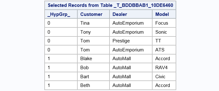
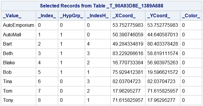
libname example sasiola host="grid001.example.com" port=10010 tag=hps;

data example.sales;
  input @1 Customer $ @7 Dealer $12. @21 Model $;
  cards;
Tina  AutoEmporium    Focus
Tony  AutoEmporium    Sonic
Tom   Prestige        TT
Tom   AutoEmporium    ATS
Blake AutoMall        Accord
Bob   AutoMall        RAV4
Bart  AutoMall        Civic
Beth  AutoMall        Accord

;;;

proc imstat data=example.sales;
  hypergroup customer dealer / vars=(model);
run;

  table example.&_TEMPLAST_;
  fetch / format;
run;
  table example.&_TEMPHYPGRP_;
  fetch / format;
run;
  table example.&_TEMPEDGES_
  fetch / format;
run;
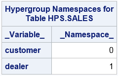
Namespace Syntax
proc imstat data=example.sales;
  hypergroup (customer, dealer) / vars=(model);
run;
Centrality Measures
Overview
Graph Centrality
Closeness Centrality
Stress Centrality
Betweenness Centrality
Centroid Centrality
Result Tables
Overview
proc imstat data=example.sales;
  hypergroup customer dealer / vars=(model);  1
run;

  table example.&_TEMPLAST_;  2
  fetch / format;
run;

  table example.&_TEMPHYPGRP_;  3
  fetch / format;
run;

  table example.&_TEMPEDGES_;  4
  fetch / format;
run;
| 1 | Because the analysis variables, customer and dealer, are specified with the simple syntax, the HYPERGROUP statement considers them both as vertices. The statement does not differentiate between customers and dealers that might have the same value. The VARS= option copies the model variable to the _TEMPLAST_ table. |
| 2 | The _TEMPLAST_ temporary table is set as the active table. The FETCH statement prints the first 20 rows from the table and formats the variables.The _TEMPLAST_ temporary table is set as the active table. |
| 3 | This is identical to the previous description except that the _TEMPHYPGRP_ temporary table is set as the active table. |
| 4 | This is identical to the previous description except that the _TEMPEDGES_ temporary table is set as the active table. |
FETCH / OUT=libref.HYPGROUPS;.
If you want to analyze the tables with clients like SAS Visual Analytics,
then use the PROMOTE statement to make it a permanent table. For metadata-aware
applications like SAS Visual Analytics, you also need to register
the table in SAS metadata.
The _TEMPLAST_ Table
-
For each row in the active table that is analyzed, subject to a WHERE clause, there is a row in the _TEMPLAST_ table.
-
The _HypGrp_ variable identifies the hypergroup number (0, 1, 2, and so on) for analysis variables.
-
The analysis variables are included in the table as well as any variables that you specify in the VARS= option.
The _TEMPHYPGRP_ Table
-
The _Value_ variable identifies the values of the hypergroup variables. These are the graph vertices names.
-
The _Index_ variable identifies each vertex index.
-
The _HypGrp_ variable identifies the hypergroup number for the vertex.
-
The _IndexH_ variable identifies a vertex index within a hypergroup subgraph.
-
The _XCoord_ and _YCoord_ variables identify the coordinates of the vertex.
-
The _Color_ variable is the index of a strongly connected component found by the graph partitioning algorithm.
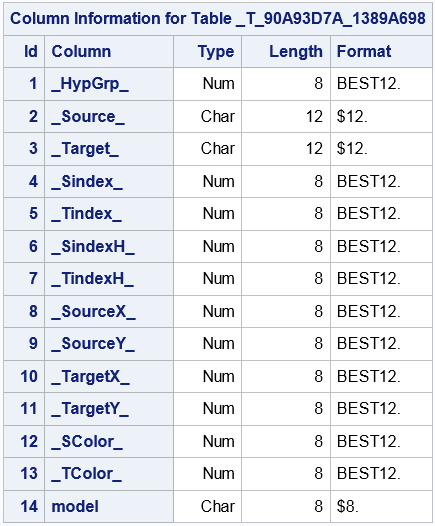
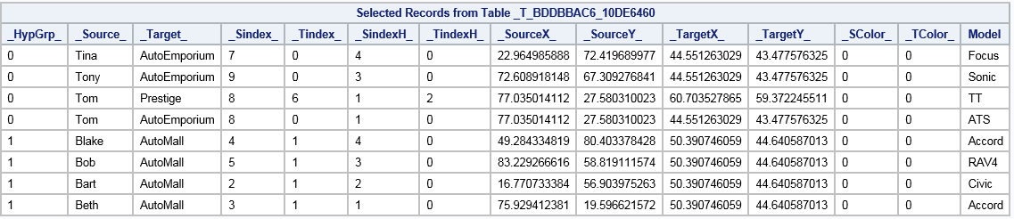
The _TEMPEDGES_ Table
-
The _HypGrp_ variable identifies the hypergroup number for analysis variables.
-
The _Source_ and _Target_ variables have the values of the vertices that each edge connects.
-
The _Sindex_ and _Tindex_ variables identify the vertex index (0, 1, 2, and so on) for the _Source_ and _Target_ variables.
-
The _SindexH_ and _TindexH_ variables identify the vertex index (0, 1, 2, and so on) for the _Source_ and _Target_ variables, within each hypergroup subgraph.
-
The _XCoordS_ and _YCoordS_variables identify the coordinates of the source vertex.
-
The _XCoordT_ and _YCoordT_ variables identify the coordinates of the target vertex.
-
The _SColor_ and _TColor_ variables identify the index to associate with the source and target vertices.
Additional Tables and Columns in Result Tables
ODS Table Names
|
ODS Table Name
|
Description
|
Option
|
|---|---|---|
|
HypGrpTables
|
Temporary hypergroup
table names
|
Default
|
|
Namespace
|
Hypergroup namespaces
for a table
|
When analysis
variables are specified with the namespace
syntax.
|