Organizing Panel Contents
Grid Dimensions and Cell Population Order
Assume you want to create
a DATAPANEL layout with one classification variable that has five
unique values. Before starting to write code, you must first decide
what grid dimensions you want to set (how many columns and rows) and
whether you want to permit empty cells in the grid. If do not want
empty cells, you must limit the grid to five cells, which gives you
two choices for the grid dimensions: five columns by one row (5x1),
or one column by five rows (1x5). If you are willing to have empty
cells in the grid, you could have several grid sizes, such as a 2x3
or a 3x2 grid.
The easiest way to specify a grid dimension is to set both the COLUMNS=
and ROWS= options to the desired number of columns and rows. If
one dimension is set, the other dimension automatically grows to accommodate
the number of classification levels. By default, COLUMNS=1, and the
ROWS= option is not set.
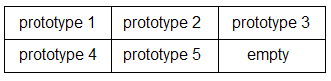
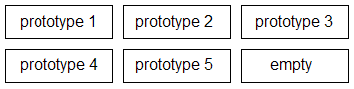
By default,
the layout uses the ORDER=ROWMAJOR setting to populate grid cells.
This specification essentially means "fill in all cells in the top
row (starting at the top left) and then continue to the next row below."
The following layout leaves the default ORDER=ROWMAJOR setting in
effect:
layout datapanel  classvars=(var) / columns=3 rows=2 ;
  layout prototype;
    ... plot statements ...
  endlayout;
endlayout;
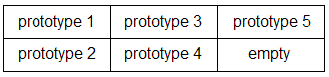
Alternatively, you can
specify ORDER=COLUMNMAJOR, which populates the grid by filling in
all cells in the left column (starting at the top), and then continuing
with the next column:
layout datapanel classvars=(var) / columns=3 rows=2 order=columnmajor ;
  layout prototype;
    ... plot statements ...
  endlayout;
endlayout;
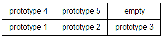
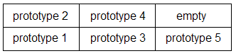
One last variation is to specify START=BOTTOMLEFT which
produces the following grids, depending on the setting for the ORDER=
option:
layout datapanel classvars=(var) / columns=3 rows=2 start=bottomleft ;
  layout prototype;
    ... plot statements ...
  endlayout;
endlayout;
layout datapanel classvars=(var) / columns=3 rows=2
    order=columnmajor start=bottomleft ;
  layout prototype;
    ... plot statements ...
  endlayout;
endlayout;
Note: The ROWS=, COLUMNS=, and
START= options are available on both the DATAPANEL and DATALATTICE
layouts. The ORDER= option is available only on the DATAPANEL layout.
If the number of unique
values of the classifiers exceeds the number of defined cells, you
automatically get as many separate panels as it takes to exhaust all
the classification levels (assuming that the PANELNUMBER= option is
not used). So if there are 17 classification levels and you define
a 2x3 grid, three panels are created (with different names), and the
last panel will have one empty cell. The effect that the classifier
values have on the panel display is illustrated in Controlling the Interactions of Classifiers.
When you specify multiple
classification variables, the crossings are always generated in a
specific way: by cycling though the last classifier, and then the
next-to-last, until all classifiers are exhausted. The following illustration
assumes that classifier A has distinct values a1 and a2, and that
classifier B has distinct values b1, b2, and b3:
layout datapanel classvars=(A B) / columns=3 rows=2 ;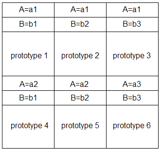
Gutters
To conserve space in
the graph, the default DATAPANEL and DATALATTICE layouts do not include
a gap between cell boundaries in the panel. In some cases, this might
cause the cell contents to appear too congested. You can add a vertical
gap between all cells with the COLUMNGUTTER= option, and you can add
a horizontal gap between all rows with the ROWGUTTER= option. If
no units are specified, pixels (PX) are assumed.
layout lattice classvars=(var) / columns=3 rows=2
    columngutter=5 rowgutter=5 ;
  layout prototype;
    ... plot statements ...
  endlayout;
endlayout;
Note that by adding
gutters, you do not increase the size of the graph. Instead, the cells
shrink to accommodate the gutters. Depending on the number of cells
in the grid and the size of the gutters, you will frequently want
to adjust the size of the graph to obtain optimal results, especially
if the cells contain complex graphs. The issues of graph size and
cell size are discussed in the following sections.
Graph Aspect Ratio
The default graph size
is 640 pixels in width and 480 pixels in height, which sets a default
aspect ratio of 4:3 (640:480). Depending on your grid size, you might
want to adjust the aspect ratio to improve the appearance of the panel.
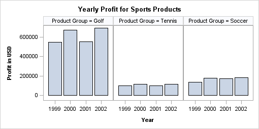
The following example uses a three column by one row grid with the
default aspect ratio:
proc template;
define statgraph onerow;
begingraph;
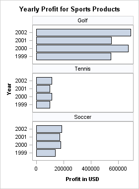
entrytitle "Yearly Profit for Sports Products";
layout datapanel classvars=(product_group) / rows=1 ;
layout prototype;
barchart x=year y=profit / stat=sum ;
endlayout;
endlayout;
endgraph;
end;
run;
proc sgrender data=sashelp.orsales template=onerow;
where product_group in ("Golf" "Tennis" "Soccer");
run;
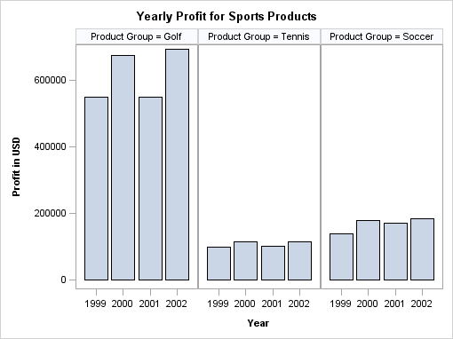
In this case, the height of the cells could be reduced
to improve the appearance. To adjust the size of the graph, use the
DESIGNHEIGHT= and/or DESIGNWIDTH= options in the BEGINGRAPH statement.
The following panel is rendered with a 2:1 aspect ratio.
begingraph / designwidth=640px designheight=320px ;
   . . .
endgraph;
IThe DESIGNWIDTH= and DESIGNHEIGHT= options set the graph size as
part of the template definition so that if you later want a larger
or smaller version of this graph, you do not have to reset the design
size and recompiling the template. Rather, you can specify either
a WIDTH= or a HEIGHT= option in the ODS GRAPHICS statement. The other
dimension is automatically computed for you, based on the aspect ratio
that is specified in the compiled template by the DESIGNWIDTH= and
DESIGNHEIGHT= options. For example, the following template produces
a 5 inch by 2.5 inch graph (the 2:1 aspect ratio is maintained).
ods graphics / reset width=5in ;

proc sgrender data=sashelp.orsales template=onerow;
  where product_group in ("Golf" "Tennis" "Soccer");
run;
Cell Size
You might think that
the panel size can be varied to be as big or small as desired. However,
problems arise as the graph size shrinks. Several adjustments in the
graph enable small images to be produced:
-
Labels in the cell headers are truncated. (The options that are available for controlling the cell header content and size are discussed in Controlling the Classification Headers.)
For example, the following
code sets a 420 pixel width for a classification panel:
ods graphics / reset width=420px ;

proc sgrender data=sashelp.orsales template=onerow;
  where product_group in ("Golf" "Tennis" "Soccer");
run;
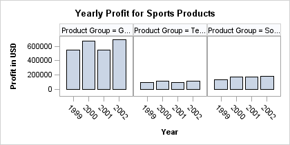
This panel is approaching
the limits of how small it can be. Reducing the size even more would
eventually produce log messages similar to the following:
Cell width 72 is smaller than the minimum cell width 100. All contents are
removed from the layout.

NOTE: Listing image output written to SGRender.png.
NOTE: There were 48 observations read from the data set SASHELP.ORSALES.
      WHERE product_group in ('Golf', 'Soccer', 'Tennis');
NOTE: PROCEDURE SGRENDER used (Total process time):
      real time           0.50 seconds
      cpu time            0.28 seconds
Although an image is
produced, it is empty. The GTL has an internal restriction on how
small a cell in the panel can be: 100 pixels by 100 pixels. Cell size
is computed after all titles, footnotes, and sidebar contents have
been established. Thus, if we had additional titles in the panel design,
log messages similar to the one just shown would be issued, even with
a larger panel size.
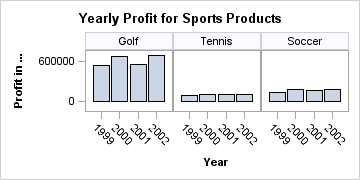
The CELLWIDTHMIN= and CELLHEIGHTMIN= options on the LAYOUT
DATAPANEL or LAYOUT DATALATTICE statements can be used to specify
smaller cell sizes than 100 pixels:
proc template;
 define statgraph onerow;
  begingraph / designwidth=360px designheight=180px;
    entrytitle "Yearly Profit for Sports Products";
    layout datapanel classvars=(product_group) / rows=1
                     headerlabeldisplay=value
                     cellwidthmin=70 cellheightmin=70 ;
      layout prototype;
        barchart x=year y=profit / stat=sum;
      endlayout;
    endlayout;
  endgraph;
 end;
run;

proc sgrender data=sashelp.orsales template=onerow;
  where product_group in ("Golf" "Tennis" "Soccer");
run;
For graph templates
that are intended for repeated use (such as the ones that are part
of other SAS products), the effort has been made to set the CELLWIDTHMIN=
and CELLHEIGHTMIN= option to the smallest values that produce a reasonable
panel. Other strategies produce smaller cells without truncating text
or resulting in other unwanted side effects. For example, you can
change the orientation of the prototype layout.
Prototype Orientation
Rather than generating
a graph with the default row orientation, you can present the same
information in a column-oriented format. To do so, you should change
the design size and also consider changing the orientation of the
prototype plot. Prototype plots with discrete axes often benefit from
a horizontal orientation because the horizontal alignment can display
discrete axis tick values without rotation or truncation (although
it might eventually thin or stagger the ticks). The following template
code sets a horizontal orientation on a prototype graph.
proc template;
 define statgraph onecol;
  begingraph / designwidth=280px designheight=380px ;
    entrytitle "Yearly Profit for Sports Products";
    layout datapanel   classvars=(product_group) / columns=1
           headerlabeldisplay=value
           cellwidthmin=85 cellheightmin=85 ;
      layout prototype;
        barchart x=year y=profit / stat=sum
                                   orient=horizontal ;
      endlayout;
    endlayout;
  endgraph;
 end;
run;

proc sgrender data=sashelp.orsales template=onecol;
  where product_group in ("Golf" "Tennis" "Soccer");
run;