The X13 Procedure
- Overview
-
Getting Started

-
SyntaxFunctional SummaryPROC X13 StatementADJUST StatementARIMA StatementAUTOMDL StatementBY StatementCHECK StatementESTIMATE StatementEVENT StatementFORECAST StatementID StatementIDENTIFY StatementINPUT StatementOUTLIER StatementOUTPUT StatementPICKMDL StatementREGRESSION StatementSEATSDECOMP StatementTABLES StatementTRANSFORM StatementUSERDEFINED StatementVAR StatementX11 Statement
-
DetailsData RequirementsMissing ValuesSAS Predefined EventsUser-Defined Regression VariablesCombined Test for the Presence of Identifiable SeasonalityComputationsPICKMDL Model SelectionSEATS DecompositionDisplayed Output, ODS Table Names, and OUTPUT Tablename KeywordsTable D 8.BUsing Auxiliary Variables to Subset Output Data SetsODS GraphicsOUT= Data SetSEATSDECOMP OUT= Data SetSpecial Data Sets
-
ExamplesARIMA Model IdentificationModel EstimationSeasonal AdjustmentRegARIMA Automatic Model SelectionAutomatic Outlier DetectionUser-Defined RegressorsMDLINFOIN= and MDLINFOOUT= Data SetsSetting Regression ParametersCreating an MDLINFO= Data Set for Use with the PICKMDL StatementIllustration of ODS GraphicsAUXDATA= Data Set
- References
Combined Test for the Presence of Identifiable Seasonality
The seasonal component of a time series,  , is defined as the intrayear variation that is repeated constantly (stable) or in an evolving fashion from year to year (moving
seasonality). If the increase in the seasonal factors from year to year is too large, then the seasonal factors introduce
distortion into the model. It is important to determine whether seasonality is identifiable without distorting the series.
, is defined as the intrayear variation that is repeated constantly (stable) or in an evolving fashion from year to year (moving
seasonality). If the increase in the seasonal factors from year to year is too large, then the seasonal factors introduce
distortion into the model. It is important to determine whether seasonality is identifiable without distorting the series.
For seasonality to be identifiable, the series should be identified as seasonal by using the "Test for the Presence of Seasonality Assuming Stability" and "Nonparametric Test for the Presence of Seasonality Assuming Stability." Also, since the presence of moving seasonality can cause distortion, it is important to evaluate the moving seasonality in conjunction with the stable seasonality to determine whether the seasonality is identifiable. The results of these tests are displayed in "F tests for Seasonality" (Table D8.A) in the X13 procedure.
The test for identifiable seasonality is performed by combining the F tests for stable and moving seasonality, along with a Kruskal-Wallis test for stable seasonality. The following description is based on Lothian and Morry (1978b). Other details can be found in Dagum (1988, 1983).
Let  and
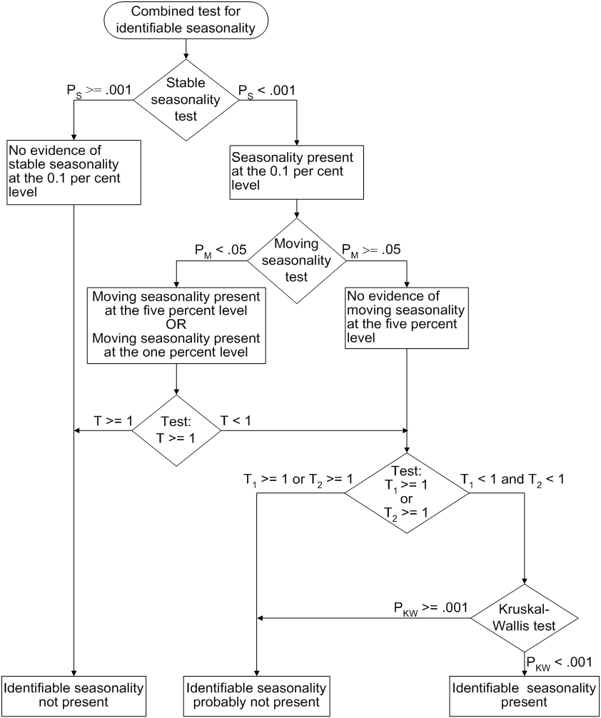
and  denote the F value for the stable and moving seasonality tests, respectively. The combined test is performed as follows (see also Figure 45.3):
-
If the null hypothesis of no stable seasonality is not rejected at the 0.10% significance level (
 ), then the series is considered to be nonseasonal. PROC X13 returns the conclusion, "Identifiable Seasonality Not Present."
-
If the null hypothesis in step 1 is rejected, then PROC X13 computes the following quantities:
![\[ T_{1} = \frac{7}{F_{s}} \]](images/etsug_x130097.png)
![\[ T_{2} = \frac{3F_{m}}{F_{s}} \]](images/etsug_x130098.png)
Let T denote the simple average of
 and
and  :
:
![\[ T = \frac{(T_{1}+T_{2})}{2} \]](images/etsug_x130101.png)
If the null hypothesis of no moving seasonality is rejected at the 5.0% significance level (
 ) and if
  , the null hypothesis of identifiable seasonality not present is not rejected and PROC X13 returns the conclusion, "Identifiable Seasonality Not Present."
-
If the null hypothesis of identifiable seasonality not present has not been accepted, but
 ,
,  , or the Kruskal-Wallis chi-squared test fails to reject at the 0.10% significance level (
 ), then PROC X13 returns the conclusion "Identifiable Seasonality Probably Not Present."
-
If the null hypotheses of no stable seasonality associated with the
 and Kruskal-Wallis chi-squared tests are rejected and if none of the combined measures described in steps 2 and 3 fail, then
the null hypothesis of identifiable seasonality not present is rejected and PROC X13 returns the conclusion "Identifiable Seasonality Present."
and Kruskal-Wallis chi-squared tests are rejected and if none of the combined measures described in steps 2 and 3 fail, then
the null hypothesis of identifiable seasonality not present is rejected and PROC X13 returns the conclusion "Identifiable Seasonality Present."
Included in the displayed output of Table D8A is the table "Summary of Results and Combined Test for the Presence of Identifiable
Seasonality." This table displays the , , and T values and the significance levels for the stable seasonality test, the moving seasonality test, and the Kruskal-Wallis test.
The last item in the table is the result of the combined test for identifiable seasonality.
Figure 45.3: Combined Seasonality Test Flowchart