The SEVERITY Procedure
- Overview
-
Getting Started

-
Syntax
-
DetailsPredefined DistributionsCensoring and TruncationParameter Estimation MethodParameter InitializationEstimating Regression EffectsLevelization of Classification VariablesSpecification and Parameterization of Model EffectsEmpirical Distribution Function Estimation MethodsStatistics of FitDefining a Severity Distribution Model with the FCMP ProcedurePredefined Utility FunctionsScoring FunctionsCustom Objective FunctionsMultithreaded ComputationInput Data SetsOutput Data SetsDisplayed OutputODS Graphics
-
ExamplesDefining a Model for Gaussian DistributionDefining a Model for the Gaussian Distribution with a Scale ParameterDefining a Model for Mixed-Tail DistributionsEstimating Parameters Using Cramér-von Mises EstimatorFitting a Scaled Tweedie Model with RegressorsFitting Distributions to Interval-Censored DataDefining a Finite Mixture Model That Has a Scale ParameterPredicting Mean and Value-at-Risk by Using Scoring FunctionsScale Regression with Rich Regression Effects
- References
An Example of Modeling Regression Effects
Consider a scenario in which the magnitude of the response variable might be affected by some regressor (exogenous or independent)
variables. The SEVERITY procedure enables you to model the effect of such variables on the distribution of the response variable
via an exponential link function. In particular, if you have k random regressor variables denoted by  (
( ), then the distribution of the response variable Y is assumed to have the form
![\[ Y \sim \exp (\sum _{j=1}^{k} \beta _ j x_ j) \cdot \mathcal{F}(\Theta ) \]](images/etsug_severity0007.png)
where  denotes the distribution of Y with parameters
  and
and  denote the regression parameters (coefficients). For the effective distribution of Y to be a valid distribution from the same parametric family as , it is necessary for to have a scale parameter. The effective distribution of Y can be written as
![\[ Y \sim \mathcal{F}(\theta , \Omega ) \]](images/etsug_severity0011.png)
where  denotes the scale parameter and
  denotes the set of nonscale parameters. The scale is affected by the regressors as
![\[ \theta = \theta _0 \cdot \exp (\sum _{j=1}^{k} \beta _ j x_ j) \]](images/etsug_severity0014.png)
where  denotes a base value of the scale parameter.
Given this form of the model, PROC SEVERITY allows a distribution to be a candidate for modeling regression effects only if it has an untransformed or a log-transformed scale parameter.
All the predefined distributions, except the lognormal distribution, have a direct scale parameter (that is, a parameter that
is a scale parameter without any transformation). For the lognormal distribution, the parameter  is a log-transformed scale parameter. This can be verified by replacing with a parameter
  , which results in the following expressions for the PDF f and the CDF F in terms of and
  , respectively, where
  denotes the CDF of the standard normal distribution:
![\[ f(x; \theta , \sigma ) = \frac{1}{x \sigma \sqrt {2 \pi }} e^{-\frac{1}{2}\left(\frac{\log (x) - \log (\theta )}{\sigma }\right)^2} \quad \text {and} \quad F(x; \theta , \sigma ) = \Phi \left(\frac{\log (x) - \log (\theta )}{\sigma }\right) \]](images/etsug_severity0019.png)
With this parameterization, the PDF satisfies the 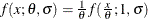 condition and the CDF satisfies the
 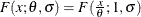 condition. This makes a scale parameter. Hence,
  is a log-transformed scale parameter and the lognormal distribution is eligible for modeling regression effects.
The following DATA step simulates a lognormal sample whose scale is decided by the values of the three regressors X1, X2, and X3 as follows:
![\[ \mu = \log (\theta ) = 1 + 0.75 \; \text {X1} - \text {X2} + 0.25 \; \text {X3} \]](images/etsug_severity0023.png)
/*----------- Lognormal Model with Regressors ------------*/
data test_sev3(keep=y x1-x3
               label='A Lognormal Sample Affected by Regressors');
   array x{*} x1-x3;
   array b{4} _TEMPORARY_ (1 0.75 -1 0.25);
   call streaminit(45678);
   label y='Response Influenced by Regressors';
   Sigma = 0.25;
   do n = 1 to 100;
      Mu = b(1); /* log of base value of scale */
      do i = 1 to dim(x);
         x(i) = rand('UNIFORM');
         Mu = Mu + b(i+1) * x(i);
      end;
      y = exp(Mu) * rand('LOGNORMAL')**Sigma;
      output;
   end;
run;
The following PROC SEVERITY step fits the lognormal, Burr, and gamma distribution models to this data. The regressors are specified in the SCALEMODEL statement. The DFMIXTURE= option in the SCALEMODEL statement specifies the method of computing the CDF estimates that are used to compute the EDF-based statistics of fit.
proc severity data=test_sev3 crit=aicc print=all;
   loss y;
   scalemodel x1-x3 / dfmixture=full;

   dist logn burr gamma;
run;
Some of the key results prepared by PROC SEVERITY are shown in Figure 30.14 through Figure 30.18. The descriptive statistics of all the variables are shown in Figure 30.14.
Figure 30.14: Summary Results for the Regression Example
The comparison of the fit statistics of all the models is shown in Figure 30.15. It indicates that the lognormal model is the best model according to each of the likelihood-based statistics, whereas the gamma model is the best model according to two of the three EDF-based statistics.
Figure 30.15: Comparison of Statistics of Fit for the Regression Example
| All Fit Statistics | ||||||||||||||
|---|---|---|---|---|---|---|---|---|---|---|---|---|---|---|
| Distribution | -2 Log Likelihood |
AIC | AICC | BIC | KS | AD | CvM | |||||||
| Logn | 187.49609 | * | 197.49609 | * | 198.13439 | * | 210.52194 | * | 0.68991 | * | 0.74299 | 0.11044 | ||
| Burr | 190.69154 | 202.69154 | 203.59476 | 218.32256 | 0.72348 | 0.73064 | 0.11332 | |||||||
| Gamma | 188.91483 | 198.91483 | 199.55313 | 211.94069 | 0.69101 | 0.72219 | * | 0.10546 | * | |||||
| Note: The asterisk (*) marks the best model according to each column's criterion. | ||||||||||||||
The distribution information and the convergence results of the lognormal model are shown in Figure 30.16. The iteration history gives you a summary of how the optimizer is traversing the surface of the log-likelihood function in its attempt to reach the optimum. Both the change in the log likelihood and the maximum gradient of the objective function with respect to any of the parameters typically approach 0 if the optimizer converges.
Figure 30.16: Convergence Results for the Lognormal Model with Regressors
The final parameter estimates of the lognormal model are shown in Figure 30.17. All the estimates are significantly different from 0. The estimate that is reported for the parameter Mu is the base value for the log-transformed scale parameter . Let  denote the observed value for regressor
 Xi. If the lognormal distribution is chosen to model Y, then the effective value of the parameter varies with the observed values of regressors as
![\[ \mu = 1.04047 + 0.65221 \, x_1 - 0.91116 \, x_2 + 0.16243 \, x_3 \]](images/etsug_severity0025.png)
These estimated coefficients are reasonably close to the population parameters (that is, within one or two standard errors).
Figure 30.17: Parameter Estimates for the Lognormal Model with Regressors
The estimates of the gamma distribution model, which is the best model according to a majority of the EDF-based statistics,
are shown in Figure 30.18. The estimate that is reported for the parameter Theta is the base value for the scale parameter . If the gamma distribution is chosen to model Y, then the effective value of the scale parameter is  .
.
Figure 30.18: Parameter Estimates for the Gamma Model with Regressors