The SEVERITY Procedure

Example 30.5 Fitting a Scaled Tweedie Model with Regressors

The Tweedie distribution is often used in the insurance industry to explain the influence of regression effects on the distribution of losses. PROC SEVERITY provides a predefined scaled Tweedie distribution (STWEEDIE) that enables you to model the influence of regression effects on the scale parameter. The scale regression model has its own advantages such as the ability to easily account for inflation effects. This example illustrates how that model can be used to evaluate the influence of regression effects on the mean of the Tweedie distribution, which is useful in problems such rate-making and pure premium modeling.

Assume a Tweedie process, whose mean $\mu$ is affected by k regression effects $x_ j$ , $j = 1, \dotsc , k$ as follows:

$\mu = \mu _0 \exp \left( \sum _{j=1}^{k} \beta _ j x_ j \right)$

where $\mu _0$ represents the base value of the mean (you can think of $\mu _0$ as $\exp (\beta _0)$ , where $\beta _0$ is the intercept). This model for the mean is identical to the popular generalized linear model for the mean with a logarithmic link function.

More interestingly, it parallels the model used by PROC SEVERITY for the scale parameter $\theta$ ,

$\theta = \theta _0 \exp \left( \sum _{j=1}^{k} \beta _ j x_ j \right)$

where $\theta _0$ represents the base value of the scale parameter. As described in the section Tweedie Distributions, for the parameter range $p \in (1,2)$ , the mean of the Tweedie distribution is given by

$\mu = \theta \lambda \frac{2-p}{p-1}$

where $\lambda$ is the Poisson mean parameter of the scaled Tweedie distribution. This relationship enables you to use the scale regression model to infer the influence of regression effects on the mean of the distribution.

Let the data set Work.Test_Sevtw contain a sample generated from a Tweedie distribution with dispersion parameter $\phi = 0.5$ , index parameter $p = 1.75$ , and the mean parameter that is affected by three regression variables x1, x2, and x3 as follows:

$\mu = 5 \: \exp (0.25 \: \text {x1} - \text {x2} + 3 \: \text {x3})$

Thus, the population values of regression parameters are $\mu _0 = 5$ , $\beta _1 = 0.25$ , $\beta _2 = -1$ , and $\beta _3 = 3$ . You can find the code used to generate the sample in the PROC SEVERITY sample program sevex05.sas.

The following PROC SEVERITY step uses the sample in Work.Test_Sevtw data set to estimate the parameters of the scale regression model for the predefined scaled Tweedie distribution (STWEEDIE) with the dual quasi-Newton (QUANEW) optimization technique:

/*--- Fit the scale parameter version of the Tweedie distribution ---*/
proc severity data=test_sevtw outest=estw covout print=all plots=none;
   loss y;
   scalemodel x1-x3;

   dist stweedie;
   nloptions tech=quanew;
run;

The dual quasi-Newton technique is used because it requires only the first-order derivatives of the objective function, and it is harder to compute reasonably accurate estimates of the second-order derivatives of Tweedie distribution’s PDF with respect to the parameters.

Some of the key results prepared by PROC SEVERITY are shown in Output 30.5.1 and Output 30.5.2. The distribution information and the convergence results are shown in Output 30.5.1.

Output 30.5.1: Convergence Results for the STWEEDIE Model with Regressors

The SEVERITY Procedure

stweedie Distribution

Distribution Information
Name	stweedie
Description	Tweedie Distribution with Scale Parameter
Distribution Parameters	3
Regression Parameters	3

Convergence Status
Convergence criterion (FCONV=2.220446E-16) satisfied.

Optimization Summary
Optimization Technique	Dual Quasi-Newton
Iterations	42
Function Calls	243
Log Likelihood	-1044.3

The final parameter estimates of the STWEEDIE regression model are shown in Output 30.5.2. The estimate that is reported for the parameter Theta is the estimate of the base value $\theta _0$ . The estimates of regression coefficients $\beta _1$ , $\beta _2$ , and $\beta _3$ are indicated by the rows of x1, x2, and x3, respectively.

Output 30.5.2: Parameter Estimates for the STWEEDIE Model with Regressors

Parameter Estimates
Parameter	Estimate	Standard Error	t Value	Approx Pr > \|t\|
Theta	0.82345	0.29281	2.81	0.0053
Lambda	16.24203	14.02459	1.16	0.2478
P	1.74930	0.22497	7.78	<.0001
x1	0.27930	0.09879	2.83	0.0050
x2	-0.76730	0.10318	-7.44	<.0001
x3	3.03183	0.10143	29.89	<.0001

If your goal is to explain the influence of regression effects on the scale parameter, then the output displayed in Output 30.5.2 is sufficient. But, if you want to compute the influence of regression effects on the mean of the distribution, then you need to do some postprocessing. Using the relationship between $\mu$ and $\theta$ , $\mu$ can be written in terms of the parameters of the STWEEDIE model as

$\mu = \theta _0 \exp \left( \sum _{j=1}^{k} \beta _ j x_ j \right) \lambda \frac{2-p}{p-1}$

This shows that the parameters $\beta _ j$ are identical for the mean and the scale model, and the base value $\mu _0$ of the mean model is

$\mu _0 = \theta _0 \lambda \frac{2-p}{p-1}$

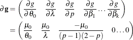
The estimate of $\mu _0$ and the standard error associated with it can be computed by using the property of the functions of maximum likelihood estimators (MLE). If $g(\Omega )$ represents a totally differentiable function of parameters $\Omega$ , then the MLE of g has an asymptotic normal distribution with mean $g(\hat{\Omega })$ and covariance $C = (\partial \mathbf{g})’ \Sigma (\partial \mathbf{g})$ , where $\hat{\Omega }$ is the MLE of $\Omega$ , $\Sigma$ is the estimate of covariance matrix of $\Omega$ , and $\partial \mathbf{g}$ is the gradient vector of g with respect to $\Omega$ evaluated at $\hat{\Omega }$ . For $\mu _0$ , the function is $g(\Omega ) = \theta _0 \lambda (2-p)/(p-1)$ . The gradient vector is

$\begin{align*} \partial \mathbf{g} & = \left( \frac{\partial g}{\partial \theta _0} \quad \frac{\partial g}{\partial \lambda } \quad \frac{\partial g}{\partial p} \quad \frac{\partial g}{\partial \beta _1} \dotsc \frac{\partial g}{\partial \beta _ k} \right) \\ & = \left( \frac{\mu _0}{\theta _0} \quad \frac{\mu _0}{\lambda } \quad \frac{-\mu _0}{(p-1)(2-p)} \quad 0 \dotsc 0 \right) \end{align*}$

You can write a DATA step that implements these computations by using the parameter and covariance estimates prepared by PROC SEVERITY step. The DATA step program is available in the sample program sevex05.sas. The estimates of $\mu _0$ prepared by that program are shown in Output 30.5.3. These estimates and the estimates of $\beta _ j$ as shown in Output 30.5.2 are reasonably close (that is, within one or two standard errors) to the parameters of the population from which the sample in Work.Test_Sevtw data set was drawn.

Output 30.5.3: Estimate of the Base Value Mu0 of the Mean Parameter

Parameter	Estimate	Standard Error	t Value	Approx Pr > \|t\|
Mu0	4.47472	0.42271	10.5858	0

Another outcome of using the scaled Tweedie distribution to model the influence of regression effects is that the regression effects also influence the variance V of the Tweedie distribution. The variance is related to the mean as $V = \phi \mu ^ p$ , where $\phi$ is the dispersion parameter. Using the relationship between the parameters TWEEDIE and STWEEDIE distributions as described in the section Tweedie Distributions, the regression model for the dispersion parameter is

$\begin{align*} \log (\phi ) & = (2-p) \log (\mu ) - \log (\lambda (2-p)) \\ & = ((2-p) \log (\mu _0) - \log (\lambda (2-p))) + (2-p) \sum _{j=1}^{k} \beta _ j x_ j \end{align*}$

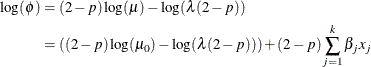
Subsequently, the regression model for the variance is

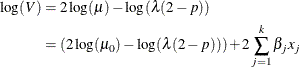
$\begin{align*} \log (V) & = 2 \log (\mu ) - \log (\lambda (2-p)) \\ & = (2 \log (\mu _0) - \log (\lambda (2-p))) + 2 \sum _{j=1}^{k} \beta _ j x_ j \end{align*}$

In summary, PROC SEVERITY enables you to estimate regression effects on various parameters and statistics of the Tweedie model.