The SEVERITY Procedure
- Overview
-
Getting Started

-
Syntax
-
DetailsPredefined DistributionsCensoring and TruncationParameter Estimation MethodParameter InitializationEstimating Regression EffectsLevelization of Classification VariablesSpecification and Parameterization of Model EffectsEmpirical Distribution Function Estimation MethodsStatistics of FitDefining a Severity Distribution Model with the FCMP ProcedurePredefined Utility FunctionsScoring FunctionsCustom Objective FunctionsMultithreaded ComputationInput Data SetsOutput Data SetsDisplayed OutputODS Graphics
-
ExamplesDefining a Model for Gaussian DistributionDefining a Model for the Gaussian Distribution with a Scale ParameterDefining a Model for Mixed-Tail DistributionsEstimating Parameters Using Cramér-von Mises EstimatorFitting a Scaled Tweedie Model with RegressorsFitting Distributions to Interval-Censored DataDefining a Finite Mixture Model That Has a Scale ParameterPredicting Mean and Value-at-Risk by Using Scoring FunctionsScale Regression with Rich Regression Effects
- References
Parameter Estimation Method
If you do not specify a custom objective function by specifying programming statements and the OBJECTIVE= option in the PROC SEVERITY statement, then PROC SEVERITY uses the maximum likelihood (ML) method to estimate the parameters of each model. A nonlinear optimization process is used to maximize the log of the likelihood function. If you specify a custom objective function, then PROC SEVERITY uses a nonlinear optimization algorithm to estimate the parameters of each model that minimize the value of your specified objective function. For more information, see the section Custom Objective Functions.
Likelihood Function
Let  and
and  denote the PDF and CDF, respectively, evaluated at x for a set of parameter values
  . Let Y denote the random response variable, and let y denote its value recorded in an observation in the input data set. Let
  and
and  denote the random variables for the left-truncation and right-truncation threshold, respectively, and let
  and
and  denote their values for an observation, respectively. If there is no left-truncation, then
  , where
  is the smallest value in the support of the distribution; so
  . If there is no right-truncation, then
  , where
  is the largest value in the support of the distribution; so
  . Let
. Let  and
and  denote the random variables for the left-censoring and right-censoring limit, respectively, and let
  and
and  denote their values for an observation, respectively. If there is no left-censoring, then
  ; so
; so  . If there is no right-censoring, then
  ; so
; so  .
.
The set of input observations can be categorized into the following four subsets within each BY group:
-
E is the set of uncensored and untruncated observations. The likelihood of an observation in E is
![\[ l_{E} = \Pr (Y=y) = f_\Theta (y) \]](images/etsug_severity0248.png)
-
 is the set of uncensored observations that are truncated. The likelihood of an observation in is
![\[ l_{E_ t} = \Pr (Y=y | t^ l < Y \leq t^ r) = \frac{f_\Theta (y)}{F_\Theta (t^ r) - F_\Theta (t^ l)} \]](images/etsug_severity0250.png)
-
C is the set of censored observations that are not truncated. The likelihood of an observation C is
![\[ l_{C} = \Pr (c^ r < Y \leq c^ l) = F_\Theta (c^ l) - F_\Theta (c^ r) \]](images/etsug_severity0251.png)
-
 is the set of censored observations that are truncated. The likelihood of an observation is
![\[ l_{C_ t} = \Pr (c^ r < Y \leq c^ l | t^ l < Y \leq t^ r) = \frac{F_\Theta (c^ l) - F_\Theta (c^ r)}{F_\Theta (t^ r) - F_\Theta (t^ l)} \]](images/etsug_severity0253.png)
Note that 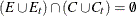 . Also, the sets and are empty when you do not specify truncation, and the sets C and are empty when you do not specify censoring.
Given this, the likelihood of the data L is as follows:

The maximum likelihood procedure used by PROC SEVERITY finds an optimal set of parameter values  that maximizes
  subject to the boundary constraints on parameter values. For a distribution dist, you can specify such boundary constraints by using the dist_LOWERBOUNDS
and dist_UPPERBOUNDS
subroutines. For more information, see the section Defining a Severity Distribution Model with the FCMP Procedure. Some aspects of the optimization process can be controlled by using the NLOPTIONS
statement.
subject to the boundary constraints on parameter values. For a distribution dist, you can specify such boundary constraints by using the dist_LOWERBOUNDS
and dist_UPPERBOUNDS
subroutines. For more information, see the section Defining a Severity Distribution Model with the FCMP Procedure. Some aspects of the optimization process can be controlled by using the NLOPTIONS
statement.
Probability of Observability and Likelihood
If you specify the probability of observability for the left-truncation, then PROC SEVERITY uses a modified likelihood function
for each truncated observation. If the probability of observability is ![$p \in (0.0, 1.0]$](images/etsug_severity0258.png) , then for each left-truncated observation with truncation threshold , there exist
, then for each left-truncated observation with truncation threshold , there exist  observations with a response variable value less than or equal to . Each such observation has a probability of
 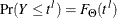 . The right-truncation and censoring information does not apply to these added observations. Thus, following the notation
of the section Likelihood Function, the likelihood of the data is as follows:
. The right-truncation and censoring information does not apply to these added observations. Thus, following the notation
of the section Likelihood Function, the likelihood of the data is as follows:
Note that the likelihood of the observations that are not left-truncated (observations in sets E and C, and observations in sets and for which  ) is not affected.
If you specify a custom objective function, then PROC SEVERITY accounts for the probability of observability only while computing the empirical distribution function estimate. The parameter estimates are affected only by your custom objective function.
Estimating Covariance and Standard Errors
PROC SEVERITY computes an estimate of the covariance matrix of the parameters by using the asymptotic theory of the maximum
likelihood estimators (MLE). If N denotes the number of observations used for estimating a parameter vector  , then the theory states that as
  , the distribution of
  , the estimate of , converges to a normal distribution with mean and covariance
  such that
  , where
 ![$\mathbf{I}(\pmb {\theta }) = -E\left[ \nabla ^2 \log (L(\pmb {\theta }))\right]$](images/etsug_severity0267.png) is the information matrix for the likelihood of the data,
is the information matrix for the likelihood of the data,  . The covariance estimate is obtained by using the inverse of the information matrix.
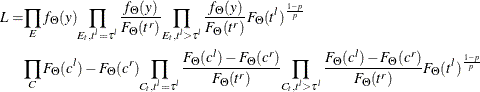
In particular, if 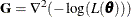 denotes the Hessian matrix of the negative of log likelihood, then the covariance estimate is computed as
![\[ \hat{\mathbf{C}} = \frac{N}{d} \mathbf{G}^{-1} \]](images/etsug_severity0270.png)
where d is a denominator that is determined by the VARDEF=
option. If VARDEF=N, then  , which yields the asymptotic covariance estimate. If VARDEF=DF, then
  , where k is number of parameters (the model’s degrees of freedom). The VARDEF=DF option is the default, because it attempts to correct
the potential bias introduced by the finite sample.
, where k is number of parameters (the model’s degrees of freedom). The VARDEF=DF option is the default, because it attempts to correct
the potential bias introduced by the finite sample.
The standard error  of the parameter
  is computed as the square root of the ith diagonal element of the estimated covariance matrix; that is,
  .
.
If you specify a custom objective function, then the covariance matrix of the parameters is still computed by inverting the
information matrix, except that the Hessian matrix  is computed as
  , where U denotes your custom objective function that is minimized by the optimizer.
Covariance and standard error estimates might not be available if the Hessian matrix is found to be singular at the end of the optimization process. This can especially happen if the optimization process stops without converging.