The SEVERITY Procedure
- Overview
-
Getting Started

-
Syntax
-
DetailsPredefined DistributionsCensoring and TruncationParameter Estimation MethodParameter InitializationEstimating Regression EffectsLevelization of Classification VariablesSpecification and Parameterization of Model EffectsEmpirical Distribution Function Estimation MethodsStatistics of FitDefining a Severity Distribution Model with the FCMP ProcedurePredefined Utility FunctionsScoring FunctionsCustom Objective FunctionsMultithreaded ComputationInput Data SetsOutput Data SetsDisplayed OutputODS Graphics
-
ExamplesDefining a Model for Gaussian DistributionDefining a Model for the Gaussian Distribution with a Scale ParameterDefining a Model for Mixed-Tail DistributionsEstimating Parameters Using Cramér-von Mises EstimatorFitting a Scaled Tweedie Model with RegressorsFitting Distributions to Interval-Censored DataDefining a Finite Mixture Model That Has a Scale ParameterPredicting Mean and Value-at-Risk by Using Scoring FunctionsScale Regression with Rich Regression Effects
- References
Example 30.9 Scale Regression with Rich Regression Effects
This example illustrates the use of regression effects that include CLASS variables and interaction effects.
Consider that you, as an actuary at an automobile insurance company, want to evaluate the effect of certain external factors
on the distribution of the severity of the losses that your policyholders incur. Such analysis can help you determine the
relative differences in premiums that you should charge to policyholders who have different characteristics. Assume that when
you collect and record the information about each claim, you also collect and record some key characteristics of the policyholder
and the vehicle that is involved in the claim. This example focuses on the following five factors: type of car, safety rating
of the car, gender of the policyholder, education level of the policyholder, and annual household income of the policyholder
(which can be thought of as a proxy for the luxury level of the car). Let these regressors be recorded in the variables CarType (1: sedan, 2: sport utility vehicle), CarSafety (scaled to be between 0 and 1, the safest being 1), Gender (1: female, 2: male), Education (1: high school graduate, 2: college graduate, 3: advanced degree holder), and Income (scaled by a factor of 1/100,000), respectively. Let the historical data about the severity of each loss be recorded in the
LossAmount variable of the Work.Losses data set. Let the data set also contain two additional variables, Deductible and Limit, that record the deductible and ground-up loss limit provisions, respectively, of the insurance policy that the policyholder
has. The limit on ground-up loss is usually derived from the payment limit that a typical insurance policy states. Deductible serves as the left-truncation variable, and Limit serves as the right-censoring variable. The SAS statements that simulate an example of the Work.Losses data set are available in the PROC SEVERITY sample program sevex09.sas.
The variables CarType, Education, and Gender each contain a known, finite set of discrete values. By specifying such variables as classification variables, you can separately
identify the effect of each level of the variable on the severity distribution. For example, you might be interested in finding
out how the magnitude of loss for a sport utility vehicle (SUV) differs from that for a sedan. This is an example of a main
effect. You might also want to evaluate how the distribution of losses that are incurred by a policyholder with a college
degree who drives a SUV differs from that of a policyholder with an advanced degree who drives a sedan. This is an example
of an interaction effect. You can include various such types of effects in the scale regression model. For more information
about the effect types, see the section Specification and Parameterization of Model Effects. Analyzing such a rich set of regression effects can help you make more accurate predictions about the losses that a new
applicant with certain characteristics might incur when he or she requests insurance for a specific vehicle, which can further
help you with ratemaking decisions.
The following PROC SEVERITY step fits the scale regression model with a lognormal distribution to data in the Work.Losses data set, and stores the model and parameter estimate information in the Work.EstStore item store:
/* Fit scale regression model with different types of regression effects */
proc severity data=losses outstore=eststore
     print=all plots=none;
   loss lossAmount / lt=deductible rc=limit;
   class carType gender education;
   scalemodel carType gender carSafety income education*carType
              income*gender carSafety*income;
   dist logn;
run;
The SCALEMODEL statement in the preceding PROC SEVERITY step includes two main effects (carType and gender), two singleton continuous effects (carSafety and income), one interaction effect (education*carType), one continuous-by-class effect (income*gender), and one polynomial continuous effect (carSafety*income). For more information about effect types, see Table 30.9.
When you specify a CLASS statement, it is recommended that you observe the "Class Level Information" table. For this example, the table is shown in Output 30.9.1. Note that if you specify BY-group processing, then the class level information might change from one BY group to the next, potentially resulting in a different parameterization for each BY group.
Output 30.9.1: Class Level Information Table
The regression modeling results for the lognormal distribution are shown in Output 30.9.2. The "Initial Parameter Values and Bounds" table is important especially because the preceding PROC SEVERITY step uses the default GLM parameterization, which is a singular parameterization—that is, it results in some redundant parameters. As shown in the table, the redundant parameters correspond to the last level of each classification variable; this correspondence is a defining characteristic of a GLM parameterization. An alternative would be to use the reference parameterization by specifying the PARAM=REFERENCE option in the CLASS statement, which does not generate redundant parameters for effects that contain CLASS variables and enables you to specify a reference level for each CLASS variable.
Output 30.9.2: Initial Values for the Scale Regression Model with Class and Interaction Effects
| Initial Parameter Values and Bounds | |||
|---|---|---|---|
| Parameter | Initial Value |
Lower Bound |
Upper Bound |
| Mu | 4.88526 | -709.78271 | 709.78271 |
| Sigma | 0.51283 | 1.05367E-8 | Infty |
| carType SUV | 0.56953 | -709.78271 | 709.78271 |
| carType Sedan | Redundant | ||
| gender Female | 0.41154 | -709.78271 | 709.78271 |
| gender Male | Redundant | ||
| carSafety | -0.72742 | -709.78271 | 709.78271 |
| income | -0.33216 | -709.78271 | 709.78271 |
| carType*education SUV AdvancedDegree | 0.31686 | -709.78271 | 709.78271 |
| carType*education SUV College | 0.66361 | -709.78271 | 709.78271 |
| carType*education SUV High School | Redundant | ||
| carType*education Sedan AdvancedDegree | -0.47841 | -709.78271 | 709.78271 |
| carType*education Sedan College | -0.25968 | -709.78271 | 709.78271 |
| carType*education Sedan High School | Redundant | ||
| income*gender Female | -0.02112 | -709.78271 | 709.78271 |
| income*gender Male | Redundant | ||
| carSafety*income | 0.13084 | -709.78271 | 709.78271 |
The convergence and optimization summary information in Output 30.9.3 indicates that the scale regression model for the lognormal distribution has converged with the default optimization technique in five iterations.
Output 30.9.3: Optimization Summary for the Scale Regression Model with Class and Interaction Effects
The "Parameter Estimates" table in Output 30.9.4 shows the distribution parameter estimates and estimates for various regression effects. You can use the estimates for effects
that contain CLASS variables to infer the relative influence of various CLASS variable levels. For example, on average, the
magnitude of losses that are incurred by the female drivers is 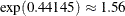 times greater than that of male drivers, and an SUV driver with an advanced degree incurs a loss that is on average
  times greater than the loss that a college-educated sedan driver incurs. Neither the continuous-by-class effect
 income*gender nor the polynomial continuous effect carSafety*income is significant in this example.
Output 30.9.4: Parameter Estimates for the Scale Regression with Class and Interaction Effects
| Parameter Estimates | ||||
|---|---|---|---|---|
| Parameter | Estimate | Standard Error |
t Value | Approx Pr > |t| |
| Mu | 5.08874 | 0.05768 | 88.23 | <.0001 |
| Sigma | 0.55774 | 0.01119 | 49.86 | <.0001 |
| carType SUV | 0.62459 | 0.04452 | 14.03 | <.0001 |
| gender Female | 0.44145 | 0.04885 | 9.04 | <.0001 |
| carSafety | -0.82942 | 0.08371 | -9.91 | <.0001 |
| income | -0.35212 | 0.07657 | -4.60 | <.0001 |
| carType*education SUV AdvancedDegree | 0.39393 | 0.07351 | 5.36 | <.0001 |
| carType*education SUV College | 0.76532 | 0.05723 | 13.37 | <.0001 |
| carType*education Sedan AdvancedDegree | -0.61064 | 0.05387 | -11.34 | <.0001 |
| carType*education Sedan College | -0.35210 | 0.03942 | -8.93 | <.0001 |
| income*gender Female | -0.01486 | 0.06629 | -0.22 | 0.8226 |
| carSafety*income | 0.07045 | 0.11447 | 0.62 | 0.5383 |
If you want to update the model when new claims data arrive, then you can potentially speed up the estimation process by specifying the OUTSTORE= item store that is created by the preceding PROC SEVERITY step as an INSTORE= item store in a new PROC SEVERITY step as follows:
/* Refit scale regression model on new data different types of regression effects */
proc severity data=withNewLosses instore=eststore
     print=all plots=all;
   loss lossAmount / lt=deductible rc=limit;
   class carType gender education;
   scalemodel carType gender carSafety income education*carType
              income*gender carSafety*income;
   dist logn;
run;
PROC SEVERITY uses the parameter estimates in the INSTORE= item store to initialize the distribution and regression parameters.