The AUTOREG Procedure
- Overview
-
Getting Started

-
Syntax
-
DetailsMissing ValuesAutoregressive Error ModelAlternative Autocorrelation Correction MethodsGARCH ModelsHeteroscedasticity- and Autocorrelation-Consistent Covariance Matrix EstimatorGoodness-of-Fit Measures and Information CriteriaTestingPredicted ValuesOUT= Data SetOUTEST= Data SetPrinted OutputODS Table NamesODS Graphics
-
Examples
- References
Example 9.8 Illustration of ODS Graphics
This example illustrates the use of ODS GRAPHICS. This is a continuation of the section Forecasting Autoregressive Error Models.
These graphical displays are requested by specifying the ODS GRAPHICS statement. For information about the graphs available in the AUTOREG procedure, see the section ODS Graphics.
The following statements show how to generate ODS GRAPHICS plots with the AUTOREG procedure. In this case, all plots are requested using the ALL option in the PROC AUTOREG statement, in addition to the ODS GRAPHICS statement. The plots are displayed in Output 9.8.1 through Output 9.8.8. Note: these plots can be viewed in the Autoreg.Model.FitDiagnosticPlots category by selecting →.
data a;
   ul = 0; ull = 0;
   do time = -10 to 36;
      u = + 1.3 * ul - .5 * ull + 2*rannor(12346);
      y = 10 + .5 * time + u;
      if time > 0 then output;
      ull = ul; ul = u;
   end;
run;

data b;
   y = .;
   do time = 37 to 46; output; end;
run;

data b;
   merge a b;
   by time;
run;
proc autoreg data=b all plots(unpack);
   model y = time / nlag=2 method=ml;
   output out=p p=yhat  pm=ytrend
                lcl=lcl ucl=ucl;
run;
Output 9.8.1: Residuals Plot

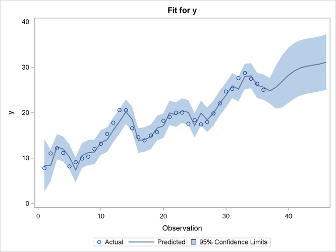
Output 9.8.2: Predicted versus Actual Plot
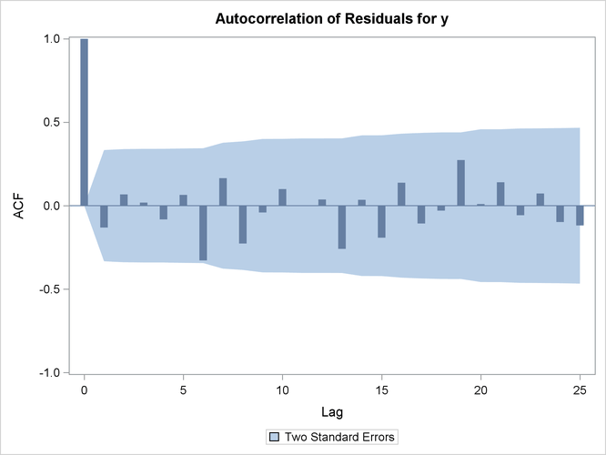
Output 9.8.3: Autocorrelation of Residuals Plot
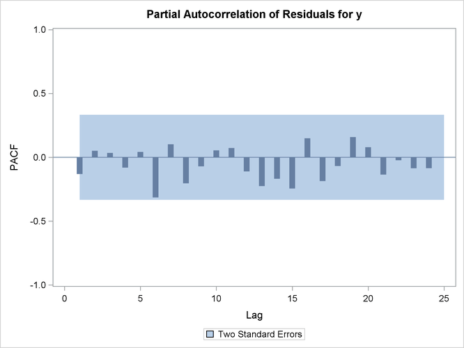
Output 9.8.4: Partial Autocorrelation of Residuals Plot
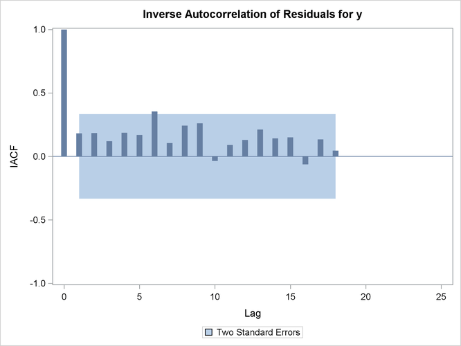
Output 9.8.5: Inverse Autocorrelation of Residuals Plot
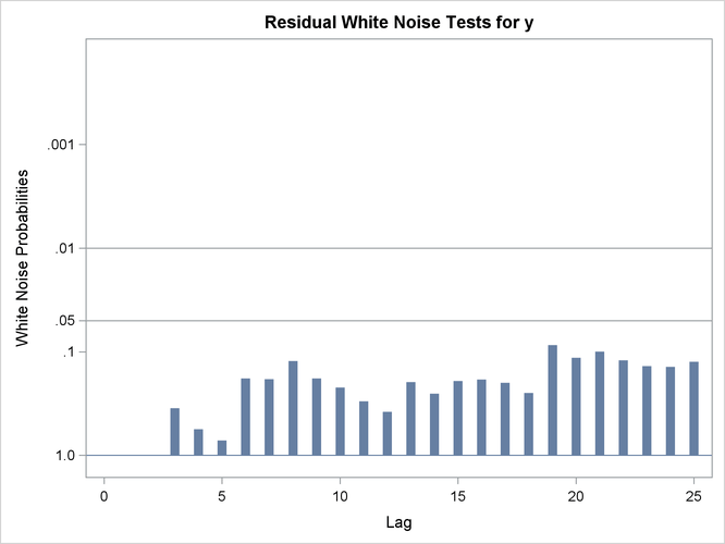
Output 9.8.6: Tests for White Noise Residuals Plot
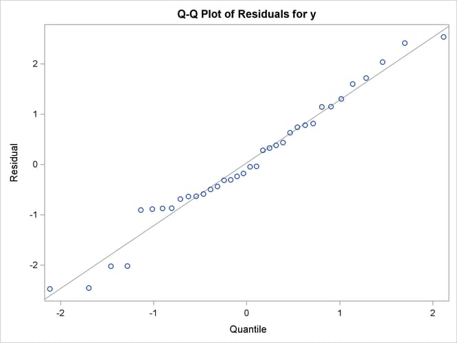
Output 9.8.7: Q-Q Plot of Residuals
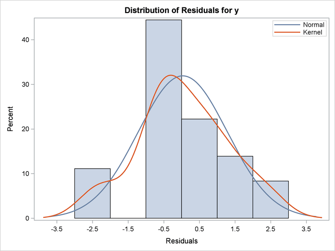
Output 9.8.8: Histogram of Residuals