PROC MDC: Testing for Homoscedasticity of the Utility Function

The MDC Procedure

Example 17.4 Testing for Homoscedasticity of the Utility Function

The conditional logit model imposes equal variances on random components of utility of all alternatives. This assumption can often be too restrictive and the calculated results misleading. This example shows several approaches to testing the homoscedasticity assumption.

The section Getting Started: MDC Procedure analyzes an HEV model by using Daganzo’s trinomial choice data and displays the HEV parameter estimates in Figure 17.15. The inverted scale estimates for mode "2" and mode "3" suggest that the conditional logit model (which imposes equal variances on random components of utility of all alternatives) might be misleading. The HEV estimation summary from that analysis is repeated in Output 17.4.1.

Output 17.4.1 HEV Estimation Summary ( $\text{[math]}$ )

Model Fit Summary
Dependent Variable	decision
Number of Observations	50
Number of Cases	150
Log Likelihood	-33.41383
Maximum Absolute Gradient	0.0000218
Number of Iterations	11
Optimization Method	Dual Quasi-Newton
AIC	72.82765
Schwarz Criterion	78.56372

You can estimate the HEV model with unit scale restrictions on all three alternatives ( $\text{[math]}$ ) with the following statements. Output 17.4.2 displays the estimation summary.

   /*-- HEV Estimation --*/
   proc mdc data=newdata;
      model decision = ttime /
               type=hev
               nchoice=3
               hev=(unitscale=1 2 3, integrate=laguerre)
               covest=hess;
      id pid;
   run;

Output 17.4.2 HEV Estimation Summary ( $\text{[math]}$ )

The MDC Procedure

Heteroscedastic Extreme Value Model Estimates

Model Fit Summary
Dependent Variable	decision
Number of Observations	50
Number of Cases	150
Log Likelihood	-34.12756
Maximum Absolute Gradient	6.7951E-9
Number of Iterations	5
Optimization Method	Dual Quasi-Newton
AIC	70.25512
Schwarz Criterion	72.16714

The test for scale equivalence (SCALE2=SCALE3=1) is performed using a likelihood ratio test statistic. The following SAS statements compute the test statistic (1.4276) and its $\text{[math]}$ -value (0.4898) from the log-likelihood values in Figure 17.4.1 and Figure 17.4.2:

   data _null_;
      /*-- test for H0: scale2 = scale3 = 1 --*/
      /*  ln L(max) = -34.1276                */
      /*  ln L(0)   = -33.4138                */
      stat = -2 * ( - 34.1276 + 33.4138 );
      df = 2;
      p_value = 1 - probchi(stat, df);
      put stat= p_value=;
   run;

The test statistic fails to reject the null hypothesis of equal scale parameters, which implies that the random utility function is homoscedastic.

A multinomial probit model also allows heteroscedasticity of the random components of utility for different alternatives. Consider the following utility function:

$\text{[math]}$

where

$\text{[math]}$

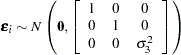This multinomial probit model is estimated by using the following program. The estimation summary is displayed in Output 17.4.3.

   /*-- Heteroscedastic Multinomial Probit --*/
   proc mdc data=newdata;
      model decision = ttime /
               type=mprobit
               nchoice=3
               unitvariance=(1 2)
               covest=hess;
      id pid;
      restrict RHO_31 = 0;
   run;

Output 17.4.3 Heteroscedastic Multinomial Probit Estimation Summary

The MDC Procedure

Multinomial Probit Estimates

Model Fit Summary
Dependent Variable	decision
Number of Observations	50
Number of Cases	150
Log Likelihood	-33.88604
Log Likelihood Null (LogL(0))	-54.93061
Maximum Absolute Gradient	5.60277E-6
Number of Iterations	8
Optimization Method	Dual Quasi-Newton
AIC	71.77209
Schwarz Criterion	75.59613
Number of Simulations	100
Starting Point of Halton Sequence	11

Next, the multinomial probit model with unit variances (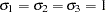 $\text{[math]}$ ) is estimated in the following statements. The estimation summary is displayed in Output 17.4.4.

   /*-- Homoscedastic Multinomial Probit --*/
   proc mdc data=newdata;
      model decision = ttime /
                type=mprobit
                nchoice=3
                unitvariance=(1 2 3)
                covest=hess;
      id pid;
      restrict RHO_21 = 0;
   run;

Output 17.4.4 Homoscedastic Multinomial Probit Estimation Summary

The MDC Procedure

Multinomial Probit Estimates

Model Fit Summary
Dependent Variable	decision
Number of Observations	50
Number of Cases	150
Log Likelihood	-34.54252
Log Likelihood Null (LogL(0))	-54.93061
Maximum Absolute Gradient	1.37303E-7
Number of Iterations	5
Optimization Method	Dual Quasi-Newton
AIC	71.08505
Schwarz Criterion	72.99707
Number of Simulations	100
Starting Point of Halton Sequence	11

The test for homoscedasticity ( $\text{[math]}$ = 1) under $\text{[math]}$ shows that the error variance is not heteroscedastic since the test statistic ( $\text{[math]}$ ) is less than $\text{[math]}$ . The marginal probability or $\text{[math]}$ -value computed in the following program from the PROBCHI function is $\text{[math]}$ .

   data _null_;
      /*-- test for H0: sigma3 = 1 --*/
      /*   ln L(max) = -33.8860      */
      /*   ln L(0)   = -34.5425      */
      stat = -2 * ( -34.5425 + 33.8860 );
      df = 1;
      p_value = 1 - probchi(stat, df);
      put stat= p_value=;
   run;

Top of Page