| The MDC Procedure |
Example 17.3 Correlated Choice Modeling
Often, it is not realistic to assume that the random components of utility for all choices are independent. This example shows the solution to the problem of correlated random components by using multinomial probit and nested logit.
To analyze correlated data, trinomial choice data (1000 observations) are created using a pseudo-random number generator by using the following statements. The random utility function is
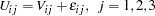 |
where
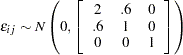 |
   /*-- generate simulated series --*/
   %let ndim = 3;
   %let nobs = 1000;

   data trichoice;
      array error{&ndim} e1-e3;
      array vtemp{&ndim} _temporary_;
      array lm{6} _temporary_ (1.4142136 0.4242641 0.9055385 0 0 1);
      retain nseed 345678 useed 223344;

      do id = 1 to &nobs;
         index = 0;
         /* generate independent normal variate */
         do i = 1 to &ndim;
            /* index of diagonal element */
            vtemp{i} = rannor(nseed);
         end;
         /* get multivariate normal variate */
         index = 0;
         do i = 1 to &ndim;
            error{i} = 0;
            do j = 1 to i;
               error{i} = error{i} + lm{index+j}*vtemp{j};
            end;
            index = index + i;
         end;
         x1 = 1.0 + 2.0 * ranuni(useed);
         x2 = 1.2 + 2.0 * ranuni(useed);
         x3 = 1.5 + 1.2 * ranuni(useed);
         util1 = 2.0 * x1 + e1;
         util2 = 2.0 * x2 + e2;
         util3 = 2.0 * x3 + e3;
         do i = 1 to &ndim;
            vtemp{i} = 0;
         end;
         if ( util1 > util2 & util1 > util3 ) then
            vtemp{1} = 1;
         else if ( util2 > util1 & util2 > util3 ) then
            vtemp{2} = 1;
         else if ( util3 > util1 & util3 > util2 ) then
            vtemp{3} = 1;
         else continue;
         /*-- first choice --*/
         x = x1;
         mode = 1;
         decision = vtemp{1};
         output;
         /*-- second choice --*/
         x = x2;
         mode = 2;
         decision = vtemp{2};
         output;
         /*-- third choice --*/
         x = x3;
         mode = 3;
         decision = vtemp{3};
         output;
      end;
   run;
First, the multinomial probit model is estimated (see the following program). Results show that standard deviation, correlation, and slope estimates are close to the parameter values. Note that 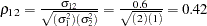 ,
,  ,
,  , and the parameter value for the variable x is 2.0. (See Output 17.3.1.)
   /*-- Trinomial Probit --*/
   proc mdc data=trichoice randnum=halton nsimul=100;
      model decision = x /
               type=mprobit
               choice=(mode 1 2 3)
               covest=op
               optmethod=qn;
      id id;
   run;
| Parameter Estimates | |||||
|---|---|---|---|---|---|
| Parameter | DF | Estimate | Standard Error |
t Value | Approx Pr > |t| |
| x | 1 | 1.7987 | 0.1202 | 14.97 | <.0001 |
| STD_1 | 1 | 1.2824 | 0.1468 | 8.74 | <.0001 |
| RHO_21 | 1 | 0.4233 | 0.1041 | 4.06 | <.0001 |
The nested model is also estimated based on a two-level decision tree (see the following program). (See Output 17.3.2.) The estimated result (see Output 17.3.3) shows that the data support the nested tree model since the estimates of the inclusive value parameters are significant and are less than 1.
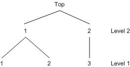
   /*-- Two-Level Nested Logit --*/
   proc mdc data=trichoice;
      model decision = x /
               type=nlogit
               choice=(mode 1 2 3)
               covest=op
               optmethod=qn;
      id id;
      utility u(1,) = x;
      nest level(1) = (1 2 @ 1, 3 @ 2),
           level(2) = (1 2 @ 1);
   run;
| Parameter Estimates | |||||
|---|---|---|---|---|---|
| Parameter | DF | Estimate | Standard Error |
t Value | Approx Pr > |t| |
| x_L1 | 1 | 2.6672 | 0.1978 | 13.48 | <.0001 |
| INC_L2G1C1 | 1 | 0.7911 | 0.0832 | 9.51 | <.0001 |
| INC_L2G1C2 | 1 | 0.7965 | 0.0921 | 8.65 | <.0001 |
Copyright © 2008 by SAS Institute Inc., Cary, NC, USA. All rights reserved.