| The MDC Procedure |
Example 17.5 Choice of Time for Work Trips: Nested Logit Analysis
This example uses sample data of 527 automobile commuters in the San Francisco Bay Area to demonstrate the use of nested logit model.
Brownstone and Small (1989) analyzed a two-level nested logit model displayed in Output 17.5.1. The probability of choosing  at level 2 is written as
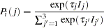 |
where  is an inclusive value and is computed as
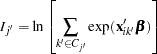 |
The probability of choosing an alternative  is denoted as
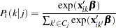 |
The full information maximum likelihood (FIML) method maximizes the following log-likelihood function:
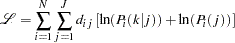 |
where  if a decision maker
  chooses , and 0 otherwise.
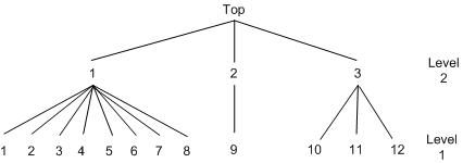
Sample data of 527 automobile commuters in the San Francisco Bay Area have been analyzed by Small (1982) and Brownstone and Small (1989). The regular time of arrival is recorded as between 42.5 minutes early and 17.5 minutes late, and indexed by 12 alternatives, using five-minute interval groups. Refer to Small (1982) for more details on these data.
The following statements estimate the two-level nested logit model:
   /*-- Two-level Nested Logit --*/
   proc mdc data=small maxit=200 outest=a;
      model decision = r15 r10 ttime ttime_cp sde sde_cp
                       sdl sdlx d2l /
               type=nlogit
               choice=(alt);
      id id;
      utility u(1, ) = r15 r10 ttime ttime_cp sde sde_cp
                       sdl sdlx d2l;
      nest level(1) = (1 2 3 4 5 6 7 8 @ 1, 9 @ 2, 10 11 12 @ 3),
           level(2) = (1 2 3 @ 1);
   run;
The estimation summary, discrete response profile, and the FIML estimates are displayed in Output 17.5.2 through Output 17.5.4.
| Model Fit Summary | |
|---|---|
| Dependent Variable | decision |
| Number of Observations | 527 |
| Number of Cases | 6324 |
| Log Likelihood | -990.81912 |
| Log Likelihood Null (LogL(0)) | -1310 |
| Maximum Absolute Gradient | 4.93868E-6 |
| Number of Iterations | 18 |
| Optimization Method | Newton-Raphson |
| AIC | 2006 |
| Schwarz Criterion | 2057 |
| Parameter Estimates | |||||
|---|---|---|---|---|---|
| Parameter | DF | Estimate | Standard Error |
t Value | Approx Pr > |t| |
| r15_L1 | 1 | 1.1034 | 0.1221 | 9.04 | <.0001 |
| r10_L1 | 1 | 0.3931 | 0.1194 | 3.29 | 0.0010 |
| ttime_L1 | 1 | -0.0465 | 0.0235 | -1.98 | 0.0474 |
| ttime_cp_L1 | 1 | -0.0498 | 0.0305 | -1.63 | 0.1028 |
| sde_L1 | 1 | -0.6618 | 0.0833 | -7.95 | <.0001 |
| sde_cp_L1 | 1 | 0.0519 | 0.1278 | 0.41 | 0.6850 |
| sdl_L1 | 1 | -2.1006 | 0.5062 | -4.15 | <.0001 |
| sdlx_L1 | 1 | -3.5240 | 1.5346 | -2.30 | 0.0217 |
| d2l_L1 | 1 | -1.0941 | 0.3273 | -3.34 | 0.0008 |
| INC_L2G1C1 | 1 | 0.6762 | 0.2754 | 2.46 | 0.0141 |
| INC_L2G1C2 | 1 | 1.0906 | 0.3090 | 3.53 | 0.0004 |
| INC_L2G1C3 | 1 | 0.7622 | 0.1649 | 4.62 | <.0001 |
Brownstone and Small (1989) also estimate the two-level nested logit model with equal scale parameter constraints,  . Replication of their model estimation is listed in the following program, and the results are displayed in Output 17.5.5 and Output 17.5.6. The parameter estimates and standard errors are almost identical to those in Brownstone and Small (1989, p. 69).
   /*-- Nested Logit with Equal Dissimilarity Parameters --*/
   proc mdc data=small maxit=200 outest=a;
      model decision = r15 r10 ttime ttime_cp sde sde_cp
                       sdl sdlx d2l /
               samescale
               type=nlogit
               choice=(alt);
      id id;
      utility u(1, ) = r15 r10 ttime ttime_cp sde sde_cp
                       sdl sdlx d2l;
      nest level(1) = (1 2 3 4 5 6 7 8 @ 1, 9 @ 2, 10 11 12 @ 3),
           level(2) = (1 2 3 @ 1);
   run;
| Model Fit Summary | |
|---|---|
| Dependent Variable | decision |
| Number of Observations | 527 |
| Number of Cases | 6324 |
| Log Likelihood | -994.39402 |
| Log Likelihood Null (LogL(0)) | -1310 |
| Maximum Absolute Gradient | 2.97172E-6 |
| Number of Iterations | 16 |
| Optimization Method | Newton-Raphson |
| AIC | 2009 |
| Schwarz Criterion | 2051 |
| Parameter Estimates | |||||
|---|---|---|---|---|---|
| Parameter | DF | Estimate | Standard Error |
t Value | Approx Pr > |t| |
| r15_L1 | 1 | 1.1345 | 0.1092 | 10.39 | <.0001 |
| r10_L1 | 1 | 0.4194 | 0.1081 | 3.88 | 0.0001 |
| ttime_L1 | 1 | -0.1626 | 0.0609 | -2.67 | 0.0076 |
| ttime_cp_L1 | 1 | 0.1285 | 0.0853 | 1.51 | 0.1319 |
| sde_L1 | 1 | -0.7548 | 0.0669 | -11.28 | <.0001 |
| sde_cp_L1 | 1 | 0.2292 | 0.0981 | 2.34 | 0.0195 |
| sdl_L1 | 1 | -2.0719 | 0.4860 | -4.26 | <.0001 |
| sdlx_L1 | 1 | -2.8216 | 1.2560 | -2.25 | 0.0247 |
| d2l_L1 | 1 | -1.3164 | 0.3474 | -3.79 | 0.0002 |
| INC_L2G1 | 1 | 0.8059 | 0.1705 | 4.73 | <.0001 |
However, the test statistic for  rejects the null hypothesis at the
  significance level since
  . The
. The  -value is computed in the following program and is equal to
  .
.
   data _null_;
      /*-- test for H0: tau1 = tau2 = tau3 --*/
      /*   ln L(max) = -990.8191             */
      /*   ln L(0)   = -994.3940             */
      stat = -2 * ( -994.3940 + 990.8191 );
      df = 2;
      p_value = 1 - probchi(stat, df);
      put stat= p_value=;
   run;
Copyright © 2008 by SAS Institute Inc., Cary, NC, USA. All rights reserved.