Hausman’s Specification Test

As discussed under multinomial and conditional logits (see the section Multinomial Logit and Conditional Logit), the odds ratios in the multinomial or conditional logits are independent of the other alternatives. This property of the logit models is often viewed as rather restrictive and provides substitution patterns that do not represent the actual relationship among choice alternatives.

This independence assumption, called Independence of Irrelevant Alternatives (IIA), can be tested with Hausman’s specification test. According to Hausman and McFadden (1984), if a subset of choice alternatives is irrelevant, it can be omitted from the sample without changing the remaining parameters systematically.

Under the null hypothesis (IIA holds), omitting the irrelevant alternatives will lead to consistent and efficient parameter estimates , while parameter estimates from the unrestricted model will be consistent but inefficient. Under the alternative, only the parameter estimates obtained from the unrestricted model will be consistent.

This example demonstrates the use of Hausman’s specification test to analyze the IIA assumption and decide on an appropriate model providing less restrictive substitution patterns (nested logit, multinomial probit). A sample data set of 527 automobile commuters in the San Francisco Bay Area is used (Small 1982). The regular time of arrival is recorded as between 42.5 minutes early and 17.5 minutes late, and indexed by 12 alternatives, using five-minute interval groups. Refer to Small (1982) for more details on these data.

Naturally, the data can be divided into three groups: commuters arriving early (alternatives 1 – 8), commuters arriving on time (alternative 9), and commuters arriving late (alternatives 10 – 12). Suppose that we want to test whether the IIA assumption holds for commuters who arrived on time (alternative 9).

Hausman’s specification test is distributed as with degrees of freedom (equal to the number of independent variables) and can be written as

where and represent parameter estimates and variance-covariance matrix from the model where the ninth alternative was omitted, and and represent parameter estimates and variance-covariance matrix from the full model. The following macro can be used to perform the IIA test for the ninth alternative.

   /*---------------------------------------------------------------
    * name: %IIA
    * note: This macro test the IIA hypothesis using the Hausman's
    *       specification test. Inputs into the macro are as follows:
    *       indata:    input data set
    *       varlist:   list of RHS variables
    *       nchoice:   number of choices for each individual
    *       choice:    list of choices
    *       nvar:      number of dependent variables
    *       nIIA:      number of choice alternatives used to test IIA
    *       IIA:       choice alternatives used to test IIA
    *       id:        ID variable
    *       decision:  0-1 LHS variable representing nchoice choices
    * purpose: Hausman's specification test
    *--------------------------------------------------------------*/
   
   %macro IIA(indata=, varlist=, nchoice=, choice= , nvar= , IIA= ,
                  nIIA=, id= , decision=);
   
      %let n=%eval(&nchoice-&nIIA);
   
      proc mdc data=&indata outest=cov covout ;
         model &decision = &varlist /
                  type=clogit
                  nchoice=&nchoice;
         id &id;
         run;
   
      data two;
         set &indata;
         if &choice in &IIA and &decision=1 then output;
      run;
   
      data two;
         set two;
         keep &id ind;
         ind=1;
      run;
   
      data merged;
         merge &indata two;
         by &id;
         if ind=1 or &choice in &IIA then delete;
      run;
   
      proc mdc data=merged outest=cov2 covout ;
         model &decision = &varlist /
                  type=clogit
                  nchoice=&n;
         id &id;
         run;
   
      proc IML;
         use cov var{_TYPE_ &varlist};
            read first into BetaU;
            read all into CovVarU where(_TYPE_='COV');
         close cov;
   
         use cov2 var{_TYPE_ &varlist};
            read first into BetaR;
            read all into CovVarR where(_TYPE_='COV');
         close cov;
   
         tmp = BetaU-BetaR;
         ChiSq=tmp*ginv(CovVarR-CovVarU)*tmp`;
         if ChiSq<0 then ChiSq=0;
         Prob=1-Probchi(ChiSq, &nvar);
         Print "Hausman Test for IIA for Variable &IIA";
         Print ChiSq Prob;
      run; quit;
   
   %mend IIA;

The following statement invokes the %IIA macro to test IIA for commuters arriving on time:

   %IIA( indata=small,
         varlist=r15 r10 ttime ttime_cp sde sde_cp sdl sdlx d2l,
         nchoice=12,
         choice=alt,
         nvar=9,
         nIIA=1,
         IIA=(9),
         id=id,
         decision=decision );

The obtained of 7.9 and the -value of 0.54 indicate that IIA does not hold for commuters arriving on time (alternative 9). In this case the following model (nested logit), which reserves a subcategory for alternative 9, might be more appropriate (Output 17.5.1):

   proc mdc data=small maxit=200 outest=a;
      model decision = r15 r10 ttime ttime_cp sde sde_cp
                       sdl sdlx d2l /
               type=nlogit
               choice=(alt);
      id id;
      utility u(1, ) = r15 r10 ttime ttime_cp sde sde_cp
                       sdl sdlx d2l;
      nest level(1) = (1 2 3 4 5 6 7 8 @ 1, 9 @ 2, 10 11 12 @ 3),
           level(2) = (1 2 3 @ 1);
   run;

Similarly, IIA could be tested for commuters arriving approximately on time (alternative 8, 9, 10), as follows:

   %IIA( indata=small,
         varlist=r15 r10 ttime ttime_cp sde sde_cp sdl sdlx d2l,
         nchoice=12,
         choice=alt,
         nvar=9,
         nIIA=3,
         IIA=(8 9 10),
         id=id,
         decision=decision );

Based on this test, independence of irrelevant alternatives is rejected for this subgroup (), and it is concluded that these three alternatives are not independent from the other nine alternatives. This finding provides a partial justification for another nested logit model, with commuters arriving approximately on time being in one subcategory.

Likelihood Ratio Test

Another specification test that can be performed is the likelihood ratio test (LR). Suppose we are interested in testing whether the nested logit model (Output 17.5.1) with three subgroups representing commuters arriving early, on time, and late is more appropriate than the standard multinomial logit. This can be done by running two logit models and calculating the LR test as follows. First, run the unrestricted nested logit model.

   /*-- Unrestricted Nested Logit --*/
   proc mdc data=small maxit=200 outest=a;
      model decision = r15 r10 ttime ttime_cp sde sde_cp
                       sdl sdlx d2l /
               type=nlogit
               choice=(alt);
      id id;
      utility u(1, ) = r15 r10 ttime ttime_cp sde sde_cp
                       sdl sdlx d2l;
      nest level(1) = (1 2 3 4 5 6 7 8 @ 1, 9 @ 2, 10 11 12 @ 3),
           level(2) = (1 2 3 @ 1);
   run;

Second, run the restricted model with inclusive value parameters constrained to one. This model, with a restriction on inclusive value parameters, is equal to the standard multinomial logit.

   /*-- Restricted Model with Inclusive Value Parameters
        Constrained to One --*/
   proc mdc data=small maxit=200 outest=a;
      model decision = r15 r10 ttime ttime_cp sde sde_cp
                       sdl sdlx d2l /
               type=nlogit
               choice=(alt);
      id id;
      utility u(1, ) = r15 r10 ttime ttime_cp sde sde_cp
                       sdl sdlx d2l;
      nest level(1) = (1 2 3 4 5 6 7 8 @ 1, 9 @ 2, 10 11 12 @ 3),
           level(2) = (1 2 3 @ 1);
      restrict INC_L2G1C1=1, INC_L2G1C2=1, INC_L2G1C3=1;
   run;

The likelihood ratio test is distributed as with degrees of freedom equal to number of restrictions imposed:

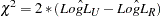where represents the log of unrestricted likelihood and is the log of restricted likelihood at the optimized solution. Unrestricted and restricted log-likelihood values can be found in the “Model Fit Summary” table (see Output 17.5.5). Calculating the LR, test we conclude that nested logit is a more appropriate model. The LR test can be used to test other types of restrictions in the nested logit setting as long as one model can be nested within another.