The HPCDM Procedure(Experimental)

Example 4.2 Using Externally Simulated Count Data
The COUNTREG procedure enables you to estimate count regression models that are based on the most commonly used discrete distributions, such as the Poisson, negative binomial (both p = 1 and p = 2), and Conway-Maxwell-Poisson distributions. PROC COUNTREG also enables you to fit zero-inflated models that are based on Poisson, negative binomial (p = 2), and Conway-Maxwell-Poisson distributions. However, there might be situations in which you want to use some other method of fitting count regression models. For example, if you are modeling the number of loss events that are incurred by two financial instruments such that there is some dependency between the two, then you might use some multivariate frequency modeling methods and simulate the counts for each instrument by using the dependency structure between the count model parameters of the two instruments. As another example, you might want to use different types of count models for different BY groups in your data; this is not possible in PROC COUNTREG in SAS/ETS 13.1 and earlier. So you need to simulate the counts for such BY groups externally. PROC HPCDM enables you to supply externally simulated counts by using the EXTERNALCOUNTS statement. PROC HPCDM then does not need to simulate the counts internally; it simulates only the severity of each loss event by using the severity model estimates in the SEVERITYEST= data set. The process is described and illustrated in the section Simulation with External Counts.
Consider that you are a bank, and as part of quantifying your operational risk, you want to estimate the aggregate loss distributions
for two lines of business, retail banking and commercial banking, by using some key risk indicators (KRIs). Assume that your
model fitting and model selection process has determined that the Poisson regression model and negative binomial regression
model are the best-fitting count models for number of loss events that are incurred in the retail banking and commercial banking
businesses, respectively. Let CorpKRI1, CorpKRI2, CbKRI1, CbKRI2, and CbKRI3 be the KRIs that are used in the count regression model of the commercial banking business, and let CorpKRI1, RbKRI1, and RbKRI2 be the KRIs that are used in the count regression model of the retail banking business. Some examples of corporate-level
KRIs (CorpKRI1 and CorpKRI2 in this example) are the ratio of temporary to permanent employees and the number of security breaches that are reported
during a year. Some examples of KRIs that are specific to the commercial banking business (CbKRI1, CbKRI2, and CbKRI3 in this example) are number of credit defaults, proportion of financed assets that are movable, and penalty claims against
your bank because of processing delays. Some examples of KRIs that are specific to the retail banking business (RbKRI1 and RbKRI2 in this example) are number of credit cards that are reported stolen, fraction of employees who have not undergone fraud
detection training, and number of forged drafts and checks that are presented in a year.
Let the severity of each loss event in the commercial banking business be dependent on two KRIs, CorpKRI1 and CbKRI2. Let the severity of each loss event in the retail banking business be dependent on three KRIs, CorpKRI2, RbKRI1, and RbKRI3. Note that for each line of business, the set of KRIs that are used for the severity model is different from the set of KRIs
that are used for the count model, although there is some overlap between the two sets. Further, the severity model for retail
banking includes a new regressor (RbKRI3) that is not used for any of the count models. Such use of different sets of KRIs for count and severity models is typical
of real-world applications.
Let the parameter estimates of the negative binomial and Poisson regression models, as determined by PROC COUNTREG, be available
in the Work.CountEstEx2NB2 and Work.CountEstEx2Poisson data sets, respectively. These data sets are produced by using the OUTEST= option in the respective PROC COUNTREG statements.
Let the parameter estimates of the best-fitting severity models, as determined by PROC SEVERITY, be available in the Work.SevEstEx2Best data set. You can find the code to prepare these data sets in the PROC HPCDM sample program hcdmex02.sas.
Now, consider that you want to estimate the distribution of the aggregate loss for a scenario, which is represented by a specific set of KRI values. The following DATA step illustrates one such scenario:
/* Generate a scenario data set for a single operating condition */
data singleScenario (keep=corpKRI1 corpKRI2 cbKRI1 cbKRI2 cbKRI3
                          rbKRI1 rbKRI2 rbKRI3);
   array x{8} corpKRI1 corpKRI2 cbKRI1 cbKRI2 cbKRI3 rbKRI1 rbKRI2 rbKRI3;
   call streaminit(5151);
   do i=1 to dim(x);
      x(i) = rand('NORMAL');
   end;
   output;
run;
The Work.SingleScenario data set contains all the KRIs that are included in the count and severity models of both business lines. Note that if you
standardize or scale the KRIs while fitting the count and severity models, then you must apply the same standardization or
scaling method to the values of the KRIs that you specify in the scenario. In this particular example, all KRIs are assumed
to be standardized.
The following DATA step uses the scenario in the Work.SingleScenario data set to simulate 10,000 replications of the number of loss events that you might observe for each business line and writes
the simulated counts to the NumLoss variable of the Work.LossCounts1 data set:
/* Simulate multiple replications of the number of loss events that
   you can expect in the scenario being analyzed */
data lossCounts1 (keep=line corpKRI1 corpKRI2 cbKRI2 rbKRI1 rbKRI3 numloss);
   array cxR{3} corpKRI1 rbKRI1 rbKRI2;
   array cbetaR{4} _TEMPORARY_;
   array cxC{5} corpKRI1 corpKRI2 cbKRI1 cbKRI2 cbKRI3;
   array cbetaC{6} _TEMPORARY_;

   retain theta;
   if _n_ = 1 then do;
      call streaminit(5151);
      * read count model estimates *;
      set countEstEx2NB2(where=(line='CommercialBanking' and _type_='PARM'));
      cbetaC(1) = Intercept;
      do i=1 to dim(cxC);
         cbetaC(i+1) = cxC(i);
      end;
      alpha = _Alpha;
      theta = 1/alpha;

      set countEstEx2Poisson(where=(line='RetailBanking' and _type_='PARM'));
      cbetaR(1) = Intercept;
      do i=1 to dim(cxR);
         cbetaR(i+1) = cxR(i);
      end;
   end;

   set singleScenario;
   do iline=1 to 2;
      if (iline=1) then line = 'CommercialBanking';
      else line = 'RetailBanking';
      do repid=1 to 10000;
         * draw from count distribution *;
         if (iline=1) then do;
            xbeta = cbetaC(1);
            do i=1 to dim(cxC);
               xbeta = xbeta + cxC(i) * cbetaC(i+1);
            end;
            Mu = exp(xbeta);
            p = theta/(Mu+theta);
            numloss = rand('NEGB',p,theta);
         end;
         else do;
            xbeta = cbetaR(1);
            do i=1 to dim(cxR);
               xbeta = xbeta + cxR(i) * cbetaR(i+1);
            end;
            numloss = rand('POISSON', exp(xbeta));
         end;
         output;
      end;
   end;
run;
The Work.LossCounts1 data set contains the NumLoss variable in addition to the KRIs that are used by the severity regression model, which are needed by PROC HPCDM to simulate
the aggregate loss.
By default, PROC HPCDM computes an aggregate loss distribution by using each of the severity models that you specify in the SEVERITYMODEL statement. However, you can restrict PROC HPCDM to use only a subset of the severity models for a given BY group by modifying the SEVERITYEST= data set to include only the estimates of the desired severity models in each BY group, as illustrated in the following DATA step:
/* Keep only the best severity model for each business line
   and set coefficients of unused regressors in each model to 0 */
data sevestEx2Best;
    set sevestEx2;
    if ((line = 'CommercialBanking' and _model_ = 'Logn')) then do;
        corpKRI2 = 0; rbKRI1 = 0; rbKRI3 = 0;
        output;
    end;
    else if ((line = 'RetailBanking' and _model_ = 'Gamma')) then do;
        corpKRI1 = 0; cbKRI2 = 0;
        output;
    end;
run;
Note that the preceding DATA step also sets the coefficients of the unused regressors in each model to 0. This is important because PROC HPCDM uses all the regressors that it detects from the SEVERITYEST= data set for each severity model.
Now, you are ready to estimate the aggregate loss distribution for each line of business by submitting the following PROC
HPCDM step, in which you specify the EXTERNALCOUNTS statement to request that external counts in the NumLoss variable of the DATA= data set be used for simulation of the aggregate loss:
/* Estimate the distribution of the aggregate loss for both
   lines of business by using the externally simulated counts */
proc hpcdm data=lossCounts1 seed=13579 print=all
           severityest=sevestEx2Best;
   by line;
   externalcounts count=numloss;
   severitymodel logn gamma;
run;
Each observation in the Work.LossCounts1 data set represents one replication of the external counts simulation process. For each such replication, the preceding PROC
HPCDM step makes as many severity draws from the severity distribution as the value of the NumLoss variable and adds the severity values from those draws to compute one sample point of the aggregate loss. The severity distribution
that is used for making the severity draws has a scale parameter value that is decided by the KRI values in the given observation
and the regression parameter values that are read from the Work.SevEstEx2Best data set.
The summary statistics and percentiles of the aggregate loss distribution for the commercial banking business, which uses
the lognormal severity model, are shown in Output 4.2.1. The "Input Data Summary" table indicates that each of the 10,000 observations in the BY group is treated as one replication
and that there are a total of 19,028 loss events produced by all the replications together. For the scenario in the Work.SingleScenario data set, you can expect the commercial banking business to incur an average aggregate loss of 653 units, as shown in the
"Sample Summary Statistics" table, and the chance that the loss will exceed 4,728 units is 0.5%, as shown in the "Sample Percentiles"
table.
Output 4.2.1: Aggregate Loss Summary for Commercial Banking Business
For the retail banking business, which uses the gamma severity model, the "Sample Percentiles" table in Output 4.2.2 indicates that the median operational loss of that business is about 71 units and the chance that the loss will exceed 380 units is about 1%.
Output 4.2.2: Aggregate Loss Percentiles for Retail Banking Business
When you conduct the simulation and estimation for a scenario that contains only one observation, you assume that the operating
environment does not change over the period of time that is being analyzed. That assumption might be valid for shorter durations
and stable business environments, but often the operating environments change, especially if you are estimating the aggregate
loss over a longer period of time. So you might want to include in your scenario all the possible operating environments that
you expect to see during the analysis time period. Each environment is characterized by its own set of KRI values. For example,
the operating conditions might change from quarter to quarter, and you might want to estimate the aggregate loss distribution
for the entire year. You start the estimation process for such scenarios by creating a scenario data set. The following DATA
step creates the Work.MultiConditionScenario data set, which consists of four operating environments, one for each quarter:
/* Generate a scenario data set for multiple operating conditions */
data multiConditionScenario (keep=opEnvId corpKRI1 corpKRI2
      cbKRI1 cbKRI2 cbKRI3 rbKRI1 rbKRI2 rbKRI3);
   array x{8} corpKRI1 corpKRI2 cbKRI1 cbKRI2 cbKRI3 rbKRI1 rbKRI2 rbKRI3;
   call streaminit(5151);
   do opEnvId=1 to 4;
      do i=1 to dim(x);
         x(i) = rand('NORMAL');
      end;
      output;
   end;
run;
All four observations of the Work.MultiConditionScenario data set together form one scenario. When simulating the external counts for such multi-entity scenarios, one replication
consists of the possible number of loss events that can occur as a result of each of the four operating environments. In any
given replication, some operating environments might not produce any loss event or all four operating environments might produce
some loss events. Assume that you use a DATA step to create the Work.LossCounts2 data set that contains, for each business line, 10,000 replications of the loss counts and that you identify each replication
by using the RepId variable. You can find the DATA step code to prepare the Work.LossCounts2 data set in the PROC HPCDM sample program hcdmex02.sas.
Output 4.2.3 shows some observations of the Work.LossCounts2 data set for each business line. For the first replication (RepId=1) of the commercial banking business, only operating environments 3 and 4 incur loss events, whereas the other environments
incur no loss events. For the second replication (RepId=2), all operating environments incur at least one loss event. For the first replication (RepId=1) of the retail banking business, operating environments 2, 3, and 4 incur two, one, and three loss events, respectively.
Output 4.2.3: Snapshot of the External Counts Data with Replication Identifier
| line | opEnvId | corpKRI1 | corpKRI2 | cbKRI2 | rbKRI1 | rbKRI3 | repid | numloss |
|---|---|---|---|---|---|---|---|---|
| CommercialBanking | 1 | 0.45224 | 0.40661 | -0.33680 | -1.08692 | -2.20557 | 1 | 0 |
| CommercialBanking | 2 | -0.03799 | 0.98670 | -0.03752 | 1.94589 | 1.22456 | 1 | 0 |
| CommercialBanking | 3 | -0.29120 | -0.45239 | 0.98855 | -0.37208 | -1.51534 | 1 | 3 |
| CommercialBanking | 4 | 0.87499 | -0.67812 | -0.04839 | -1.44881 | 0.78221 | 1 | 1 |
| CommercialBanking | 1 | 0.45224 | 0.40661 | -0.33680 | -1.08692 | -2.20557 | 2 | 2 |
| CommercialBanking | 2 | -0.03799 | 0.98670 | -0.03752 | 1.94589 | 1.22456 | 2 | 5 |
| CommercialBanking | 3 | -0.29120 | -0.45239 | 0.98855 | -0.37208 | -1.51534 | 2 | 12 |
| CommercialBanking | 4 | 0.87499 | -0.67812 | -0.04839 | -1.44881 | 0.78221 | 2 | 12 |
| RetailBanking | 1 | 0.45224 | 0.40661 | -0.33680 | -1.08692 | -2.20557 | 1 | 0 |
| RetailBanking | 2 | -0.03799 | 0.98670 | -0.03752 | 1.94589 | 1.22456 | 1 | 2 |
| RetailBanking | 3 | -0.29120 | -0.45239 | 0.98855 | -0.37208 | -1.51534 | 1 | 1 |
| RetailBanking | 4 | 0.87499 | -0.67812 | -0.04839 | -1.44881 | 0.78221 | 1 | 3 |
| RetailBanking | 1 | 0.45224 | 0.40661 | -0.33680 | -1.08692 | -2.20557 | 2 | 2 |
| RetailBanking | 2 | -0.03799 | 0.98670 | -0.03752 | 1.94589 | 1.22456 | 2 | 2 |
| RetailBanking | 3 | -0.29120 | -0.45239 | 0.98855 | -0.37208 | -1.51534 | 2 | 0 |
| RetailBanking | 4 | 0.87499 | -0.67812 | -0.04839 | -1.44881 | 0.78221 | 2 | 1 |
You can now use this simulated count data to estimate the distribution of the aggregate loss that is incurred in all four
operating environments by submitting the following PROC HPCDM step, in which you specify the replication identifier variable
RepId in the ID= option of the EXTERNALCOUNTS statement:
/* Estimate the distribution of the aggregate loss for both
   lines of business by using the externally simulated counts
   for the multiple operating environments */
proc hpcdm data=lossCounts2 seed=13579 print=all
           severityest=sevestEx2Best plots=density;
   by line;
   distby repid;
   externalcounts count=numloss id=repid;
   severitymodel logn gamma;
run;
Note that when you specify the ID= variable in the EXTERNALCOUNTS statement, you must also specify that variable in the DISTBY
statement. Within each BY group, for each value of the RepId variable, one point of the aggregate loss sample is simulated by using the process that is described in the section Simulation with External Counts.
The summary statistics and percentiles of the distribution of the aggregate loss, which is the aggregate of the losses across all four operating environments, are shown in Output 4.2.4 for the commercial banking business. The "Input Data Summary" table indicates that there are 10,000 replications in the BY group and that a total of 145,721 loss events are generated across all replications. The "Sample Percentiles" table indicates that you can expect a median aggregate loss of 4,460 units and a worst-case loss, as defined by the 99.5th percentile, of 16,304 units from the commercial banking business when you combine losses that result from all four operating environments.
Output 4.2.4: Aggregate Loss Summary for the Commercial Banking Business in Multiple Operating Environments
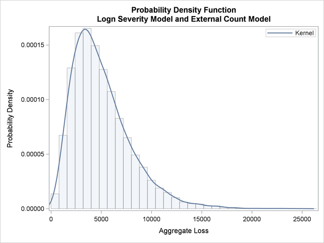
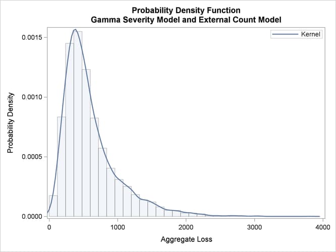
The probability density functions of the aggregate loss for the commercial and retail banking businesses are shown in Output 4.2.5. In addition to the difference in scales of the losses in the two businesses, you can see that the aggregate loss that is incurred in the commercial banking business has a heavier right tail than the aggregate loss that is incurred in the retail banking business.
Output 4.2.5: Density Plots of the Aggregate Losses for Commercial Banking (left) and Retail Banking (right) Businesses
|
|
|