The IRT Procedure
-
Overview

- Getting Started
-
Syntax
-
DetailsNotation for the Item Response Theory ModelAssumptionsPROC IRT Contrasted with Other SAS ProceduresResponse ModelsMarginal LikelihoodApproximating the Marginal LikelihoodMaximizing the Marginal LikelihoodFactor Score EstimationModel and Item FitItem and Test informationMissing ValuesOutput Data SetsODS Table NamesODS Graphics
-
Examples
- References
Example 65.1 Unidimensional IRT Models
This example shows you the features that PROC IRT provides for unidimensional analysis. The data set comes from the 1978 Quality of American Life Survey. The survey was administered to a sample of all US residents aged 18 years and older in 1978. In this survey, subjects were asked to rate their satisfaction with many different aspects of their lives. This example selects eight items. These items are designed to measure people’s satisfaction in the following areas on a seven-point scale: community, neighborhood, dwelling unit, life in the United States, amount of education received, own health, job, and how spare time is spent. For illustration purposes, the first five items are dichotomized and the last three items are collapsed into three levels.
The following DATA step creates the data set IrtUni.
data IrtUni;
   input item1-item8 @@;
   datalines;
1 0 0 0 1 1 2 1 1 1 1 1 1 3 3 3 0 1 0 0 1 1 1 1 1 0 0 1 0 1 2 3 0 0 0
0 0 1 1 1 1 0 0 1 0 1 3 3 0 0 0 0 0 1 1 3 0 0 1 0 0 1 2 2 0 1 0 0 1 1

   ... more lines ...

3 3 0 1 0 0 1 2 2 1
;
Because all the items are designed to measure subjects’ satisfaction in different aspects of their lives, it is reasonable to start with a unidimensional IRT model. The following statements fit such a model by using several user-specified options:
ods graphics on;
proc irt data=IrtUni link=probit pinitial itemstat polychoric
   itemfit plots=(icc polychoric);
   var item1-item8;
   model item1-item4/resfunc=twop, item5-item8/resfunc=graded;
run;
The ODS GRAPHICS ON statement invokes the ODS Graphics environment and displays the plots, such as the item characteristic curve plot. For more information about ODS Graphics, see Chapter 21: Statistical Graphics Using ODS.
The first option is the LINK= option, which specifies that the link function be the probit link. Next, you request initial parameter estimates by using the PINITIAL option. Item fit statistics are displayed using the ITEMFIT option. In the PROC IRT statement, you can use the PLOTS option to request different plots. In this example, you request item characteristic curves by using the PLOTS=ICC option.
In this example, you use the MODEL
statement to specify different response models for different items. The specifications in the MODEL
statement suggest that the first four items, item1 to item4, are fitted using the two-parameter model, whereas the last four items, item5 to item8, are fitted using the graded response model.
Output 65.1.1 displays two tables. From the "Modeling Information" table, you can observe that the link function has changed from the default
LOGIT link to the specified PROBIT link. The "Item Information" table shows that item1 to item5 each have two levels and item6 to item8 each have three levels. The last column shows the raw values of these different levels.
Output 65.1.1: Basic Information
Output 65.1.2 displays the classical item statistics table, which include the item means, item-total correlations, adjusted item-total correlations, and item means for i ordered groups of observations or individuals. You can produce this table by specifying the ITEMSTAT option in the PROC IRT statement.
Output 65.1.2: Classical Item Statistics
| Item Statistics | |||||||
|---|---|---|---|---|---|---|---|
| Item | Mean | Item-Total Correlations | Means | ||||
| Unadjusted | Adjusted | G1 (N=132) |
G2 (N=139) |
G3 (N=119) |
G4 (N=110) |
||
| item1 | 0.42400 | 0.57595 | 0.43291 | 0.11364 | 0.26619 | 0.53782 | 0.87273 |
| item2 | 0.34400 | 0.53837 | 0.39480 | 0.06818 | 0.19424 | 0.45378 | 0.74545 |
| item3 | 0.38800 | 0.51335 | 0.36132 | 0.09091 | 0.30216 | 0.47899 | 0.75455 |
| item4 | 0.41000 | 0.44559 | 0.28197 | 0.16667 | 0.30935 | 0.47899 | 0.75455 |
| item5 | 0.63000 | 0.43591 | 0.27436 | 0.32576 | 0.64029 | 0.71429 | 0.89091 |
| item6 | 1.82800 | 0.50955 | 0.24040 | 1.34848 | 1.66187 | 1.98319 | 2.44545 |
| item7 | 2.04200 | 0.65163 | 0.41822 | 1.30303 | 1.97842 | 2.35294 | 2.67273 |
| item8 | 2.18600 | 0.66119 | 0.43254 | 1.40909 | 2.15827 | 2.50420 | 2.80909 |
| Total N=500, Cronbach Alpha=0.6482 | |||||||
PROC IRT produces the "Eigenvalues of the Polychoric Correlation Matrix" table in Output 65.1.3 by default. You can use these eigenvalues to assess the dimension of latent factors. For this example, the fact that only the first eigenvalue is greater than 1 suggests that a one-factor model for the items is reasonable.
Output 65.1.3: Eigenvalues of Polychoric Correlations
| Eigenvalues of the Polychoric Correlation Matrix | ||||
|---|---|---|---|---|
| Eigenvalue | Difference | Proportion | Cumulative | |
| 1 | 3.11870486 | 2.12497677 | 0.3898 | 0.3898 |
| 2 | 0.99372809 | 0.10025986 | 0.1242 | 0.5141 |
| 3 | 0.89346823 | 0.03116998 | 0.1117 | 0.6257 |
| 4 | 0.86229826 | 0.10670185 | 0.1078 | 0.7335 |
| 5 | 0.75559640 | 0.17795713 | 0.0944 | 0.8280 |
| 6 | 0.57763928 | 0.10080017 | 0.0722 | 0.9002 |
| 7 | 0.47683911 | 0.15511333 | 0.0596 | 0.9598 |
| 8 | 0.32172578 | 0.0402 | 1.0000 | |
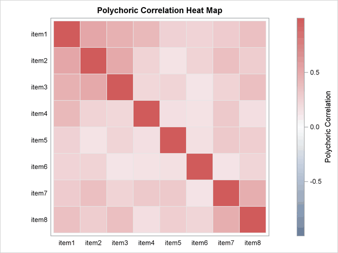
To get an overall idea of the correlations among all the items in the analysis, you can request the polychoric correlation matrix and the corresponding heat map. When you have a large number of items in the analysis, the heat map is especially useful to help you find patterns among these items. To produce the polychoric correlation matrix, specify the POLYCHORIC option in the PROC IRT statement. Specify PLOTS=POLYCHORIC to get the heat map for the polychoric correlation matrix. Output 65.1.4 includes the polychoric correlation table for this example, and Output 65.1.5 includes the heat map.
Output 65.1.4: Polychoric Correlation Matrix
| Polychoric Correlation Matrix | ||||||||
|---|---|---|---|---|---|---|---|---|
| item1 | item2 | item3 | item4 | item5 | item6 | item7 | item8 | |
| item1 | 1.0000 | 0.5333 | 0.4663 | 0.4181 | 0.2626 | 0.2512 | 0.3003 | 0.3723 |
| item2 | 0.5333 | 1.0000 | 0.5183 | 0.2531 | 0.1543 | 0.2545 | 0.3757 | 0.2910 |
| item3 | 0.4663 | 0.5183 | 1.0000 | 0.2308 | 0.2467 | 0.1455 | 0.2561 | 0.3771 |
| item4 | 0.4181 | 0.2531 | 0.2308 | 1.0000 | 0.1755 | 0.1607 | 0.3181 | 0.1825 |
| item5 | 0.2626 | 0.1543 | 0.2467 | 0.1755 | 1.0000 | 0.1725 | 0.3156 | 0.2846 |
| item6 | 0.2512 | 0.2545 | 0.1455 | 0.1607 | 0.1725 | 1.0000 | 0.1513 | 0.2404 |
| item7 | 0.3003 | 0.3757 | 0.2561 | 0.3181 | 0.3156 | 0.1513 | 1.0000 | 0.4856 |
| item8 | 0.3723 | 0.2910 | 0.3771 | 0.1825 | 0.2846 | 0.2404 | 0.4856 | 1.0000 |
Output 65.1.5: Polychoric Correlation Heat Map
The PINITIAL option in the PROC IRT statement displays the "Initial Item Parameter Estimates" table, shown in Output 65.1.6.
Output 65.1.6: Initial Parameter Estimates
| Initial Item Parameter Estimates | |||
|---|---|---|---|
| Response Model |
Item | Parameter | Estimate |
| TwoP | item1 | Difficulty | 0.26428 |
| Slope | 1.05346 | ||
| item2 | Difficulty | 0.58640 | |
| Slope | 0.93973 | ||
| item3 | Difficulty | 0.44607 | |
| Slope | 0.82826 | ||
| item4 | Difficulty | 0.50157 | |
| Slope | 0.50906 | ||
| Graded | item5 | Threshold 1 | -0.86792 |
| Slope | 0.41380 | ||
| item6 | Threshold 1 | -0.59512 | |
| Threshold 2 | 2.00678 | ||
| Slope | 0.36063 | ||
| item7 | Threshold 1 | -0.90743 | |
| Threshold 2 | 0.69335 | ||
| Slope | 0.64191 | ||
| item8 | Threshold 1 | -1.18209 | |
| Threshold 2 | 0.26959 | ||
| Slope | 0.67591 | ||
Output 65.1.7 includes tables that are related to the optimization. The "Optimization Information" table shows that the log likelihood
is approximated by using seven adaptive Gauss-Hermite quadrature points and then maximized by using the quasi-Newton algorithm.
The number of free parameters in this example is 19. The "Iteration History" table shows the number of function evaluations,
the objective function (– likelihood divided by number of subjects) values, the objective function change, and the maximum gradient for each iteration.
This information is very useful in monitoring the optimization status. Output 65.1.7 shows the convergence status at the bottom. The optimization converges according to the GCONV=0.00000001 criterion.
likelihood divided by number of subjects) values, the objective function change, and the maximum gradient for each iteration.
This information is very useful in monitoring the optimization status. Output 65.1.7 shows the convergence status at the bottom. The optimization converges according to the GCONV=0.00000001 criterion.
Output 65.1.7: Optimization Information
| Iteration History | |||||
|---|---|---|---|---|---|
| Cycles | Iteration | Evaluations | Objective Function |
Function Change |
Max Abs Gradient |
| 0 | 0 | 2 | 6.19423744 | 0.015499 | |
| 0 | 1 | 5 | 6.19269765 | -0.00153979 | 0.005785 |
| 0 | 2 | 8 | 6.19256563 | -0.00013202 | 0.003812 |
| 0 | 3 | 10 | 6.19249848 | -0.00006716 | 0.003284 |
| 0 | 4 | 12 | 6.19245354 | -0.00004493 | 0.004647 |
| 0 | 5 | 15 | 6.19243615 | -0.00001739 | 0.001284 |
| 0 | 6 | 18 | 6.19242917 | -0.00000698 | 0.000491 |
| 0 | 7 | 21 | 6.19242859 | -0.00000058 | 0.000192 |
| 0 | 8 | 24 | 6.19242845 | -0.00000013 | 0.000104 |
| 0 | 9 | 27 | 6.19242842 | -0.00000004 | 0.000051 |
| 0 | 10 | 30 | 6.19242841 | -0.00000001 | 0.000011 |
| 1 | 0 | 2 | 6.19242841 | 0.000011 | |
| 1 | 1 | 5 | 6.19242841 | -0.00000000 | 6.365E-6 |
Output 65.1.8 displays the model fit and item fit statistics. Note that the item fit statistics apply only to the binary items. That is
why these fit statistics are missing for item6 to item8.
Output 65.1.8: Fit Statistics
| Item Fit Statistics | ||||||
|---|---|---|---|---|---|---|
| Response Model |
Item | DF | Pearson Chi-Square |
Pr > P ChiSq | LR Chi-Square |
Pr > LR ChiSq |
| TwoP | item1 | 8 | 34.16711 | <.0001 | 49.39962 | <.0001 |
| item2 | 8 | 30.34805 | 0.0002 | 37.53073 | <.0001 | |
| item3 | 8 | 27.54621 | 0.0006 | 36.34596 | <.0001 | |
| item4 | 8 | 22.76082 | 0.0037 | 26.13525 | 0.0010 | |
| Graded | item5 | 8 | 18.32269 | 0.0189 | 19.68379 | 0.0116 |
| item6 | 0 | . | . | . | . | |
| item7 | 0 | . | . | . | . | |
| item8 | 0 | . | . | . | . | |
The last table for this example is the "Item Parameter Estimates " table in Output 65.1.9. This table contains parameter estimates, standard errors, and p-values. These p-values suggest that all the parameters are significantly different from zero.
Output 65.1.9: Parameter Estimates
| Item Parameter Estimates | |||||
|---|---|---|---|---|---|
| Response Model |
Item | Parameter | Estimate | Standard Error |
Pr > |t| |
| TwoP | item1 | Difficulty | 0.27339 | 0.08301 | 0.0005 |
| Slope | 0.98378 | 0.14144 | <.0001 | ||
| item2 | Difficulty | 0.60268 | 0.10047 | <.0001 | |
| Slope | 0.90006 | 0.13111 | <.0001 | ||
| item3 | Difficulty | 0.46111 | 0.10062 | <.0001 | |
| Slope | 0.79520 | 0.11392 | <.0001 | ||
| item4 | Difficulty | 0.50687 | 0.14411 | 0.0002 | |
| Slope | 0.50430 | 0.08567 | <.0001 | ||
| Graded | item5 | Threshold | -0.79749 | 0.18707 | <.0001 |
| Slope | 0.45386 | 0.08238 | <.0001 | ||
| item6 | Threshold 1 | -0.59135 | 0.19857 | 0.0015 | |
| Threshold 2 | 2.02705 | 0.39594 | <.0001 | ||
| Slope | 0.35770 | 0.06777 | <.0001 | ||
| item7 | Threshold 1 | -0.82132 | 0.12753 | <.0001 | |
| Threshold 2 | 0.64440 | 0.11431 | <.0001 | ||
| Slope | 0.72675 | 0.09313 | <.0001 | ||
| item8 | Threshold 1 | -1.08126 | 0.14132 | <.0001 | |
| Threshold 2 | 0.25165 | 0.09535 | 0.0042 | ||
| Slope | 0.76384 | 0.09754 | <.0001 | ||
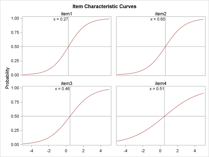
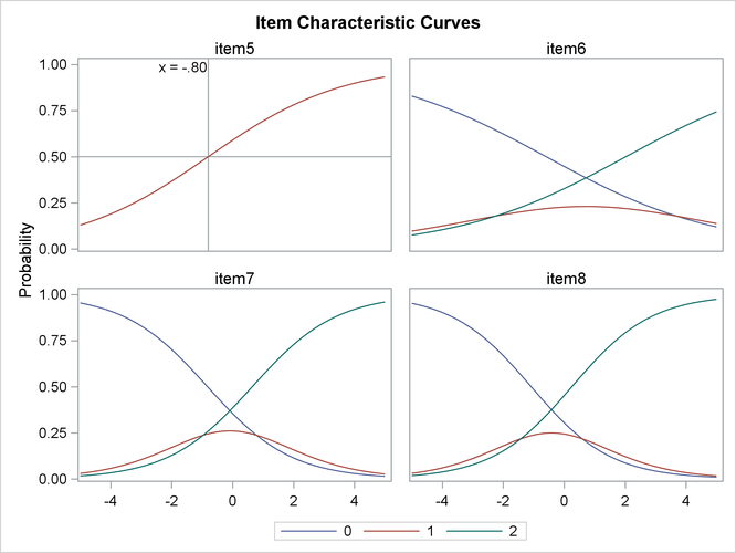
Item characteristic curves (ICC) are also produced in this example. By default, these ICC plots are displayed in panels. To display an individual ICC plot for each item, use the UNPACK suboption in the PLOTS= option in the PROC IRT statement.
Output 65.1.10: ICC Plots
Now, suppose your research hypothesis includes some equality constraints on the model parameters—for example, the slopes for the first four items are equal. Such equality constraints can be specified easily by using the EQUALITY statement. In the following example, the slope parameters of the first four items are equal:
proc irt data=IrtUni;
   var item1-item8;
   model item1-item4/resfunc=twop, item5-item8/resfunc=graded;
   equality item1-item4/parm=[slope];
run;
To estimate the factor score for each subject and add these scores to the original data set, you can use the OUT=
option in the PROC IRT
statement. PROC IRT provides three factor score estimation methods: maximum likelihood (ML), maximum a posteriori (MAP),
and expected a posteriori (EAP). You can choose an estimation method by using the SCOREMETHOD=
option in the PROC IRT
statement. The default method is maximum a posteriori. In the following, factor scores along with the original data are saved
to a SAS data set called IrtUniFscore:
proc irt data=IrtUni out=IrtUniFscore;
   var item1-item8;
   model item1-item4/resfunc=twop,
         item5-item8/resfunc=graded;
   equality item1-item4/parm=[slope];
run;
Sometimes you might find it useful to sort the items based on the estimated difficulty or slope parameters. You can do this by outputting the ODS tables for the estimates into data sets and then sorting the items by using PROC SORT. A simulated data set is used to show the steps.
The following DATA step creates the data set IrtSimu:
data IrtSimu;
   input item1-item25 @@;
   datalines;
1 1 1 0 1 1 0 0 1 1 0 0 0 0 1 0 1 1 1 0 0 0 1 0 1 1 1 1 1 1 0 1 1 0 0
0 0 0 0 0 1 1 0 0 0 1 1 1 1 0 1 1 1 1 1 1 1 1 1 1 1 1 1 1 1 1 1 1 1 1
1 1 1 1 1 1 1 1 1 0 0 0 0 0 0 0 0 1 0 0 0 1 0 0 0 0 0 1 0 0 1 1 1 1 1
1 1 1 1 1 1 1 1 1 1 1 1 1 1 1 1 1 1 1 1 1 0 0 1 0 0 0 1 1 0 0 0 0 0 0
0 1 1 1 0 0 0 0 0 0 1 1 1 1 1 1 1 1 0 1 0 0 0 1 0 1 1 0 1 1 0 0 1 1 0
1 0 0 1 1 0 0 0 1 0 0 0 0 0 0 0 1 0 1 0 1 0 1 0 0 1 1 1 1 1 1 1 1 1 1
1 1 1 1 1 0 1 1 1 1 1 1 1 1 1 1 1 1 1 1 1 1 1 1 1 1 1 1 0 0 1 1 1 1 1
1 1 1 1 1 1 1 1 1 1 1 1 1 1 1 1 1 0 1 0 1 1 1 0 1 1 1 1 1 1 0 1 0 1 1

   ... more lines ...

1 1 0 1 1 1 1 1 1 1 0 1 1 0 0 0 1 1 0 1 1 1 1 1 1 0 0 1 0 1 0 1 0 0 0
0 0 0 0 0 0 0 0 1 1 1 1 1 1 0 1 1 1 1 1 1 1 1 1 1 1 1 0 1 0 1 1 1 1 1
1 1 1 1 1 1 1 1 1 1 1 1 1 1 1 1 1 0 1 1 1 1 1 1 1 1 1 1 1 1 1 1 1 1 1
1 1 1 1 1 1 1 1 0 0 1 1 1 0 1 1 1 1 1 1
;
First, you build the model and output the parameter estimates table into a SAS data set by using the ODS OUTPUT statement:
proc irt data=IrtSimu link=probit;
   var item1-item25;
   ods output ParameterEstimates=ParmEst;
run;
Output 65.1.11 shows the "Item Parameter Estimates" table. Notice that the difficulty and slope parameters are in the same column. The reason for this is to avoid having an extremely wide table when each item has a lot of parameters.
Output 65.1.11: Basic Information
| Item Parameter Estimates | ||||
|---|---|---|---|---|
| Item | Parameter | Estimate | Standard Error |
Pr > |t| |
| item1 | Difficulty | -1.32606 | 0.09788 | <.0001 |
| Slope | 1.44114 | 0.16076 | <.0001 | |
| item2 | Difficulty | -0.99731 | 0.07454 | <.0001 |
| Slope | 1.82041 | 0.18989 | <.0001 | |
| item3 | Difficulty | -1.25020 | 0.08981 | <.0001 |
| Slope | 1.58601 | 0.17477 | <.0001 | |
| item4 | Difficulty | -1.09617 | 0.07748 | <.0001 |
| Slope | 1.86641 | 0.20431 | <.0001 | |
| item5 | Difficulty | -1.07894 | 0.07806 | <.0001 |
| Slope | 1.78216 | 0.19062 | <.0001 | |
| item6 | Difficulty | -0.95086 | 0.09402 | <.0001 |
| Slope | 1.04073 | 0.10267 | <.0001 | |
| item7 | Difficulty | -0.65080 | 0.06949 | <.0001 |
| Slope | 1.45220 | 0.13450 | <.0001 | |
| item8 | Difficulty | -0.76378 | 0.07611 | <.0001 |
| Slope | 1.30280 | 0.12210 | <.0001 | |
| item9 | Difficulty | -0.72285 | 0.07058 | <.0001 |
| Slope | 1.50546 | 0.14220 | <.0001 | |
| item10 | Difficulty | -0.50731 | 0.06125 | <.0001 |
| Slope | 1.82144 | 0.17133 | <.0001 | |
| item11 | Difficulty | -0.01272 | 0.06470 | 0.4221 |
| Slope | 1.26073 | 0.11260 | <.0001 | |
| item12 | Difficulty | 0.04106 | 0.05584 | 0.2310 |
| Slope | 2.01818 | 0.19994 | <.0001 | |
| item13 | Difficulty | 0.16143 | 0.06878 | 0.0095 |
| Slope | 1.12998 | 0.10180 | <.0001 | |
| item14 | Difficulty | 0.01159 | 0.05670 | 0.4190 |
| Slope | 1.88723 | 0.18049 | <.0001 | |
| item15 | Difficulty | 0.07250 | 0.07360 | 0.1623 |
| Slope | 0.96283 | 0.09036 | <.0001 | |
| item16 | Difficulty | -0.81425 | 0.07932 | <.0001 |
| Slope | 1.25217 | 0.11866 | <.0001 | |
| item17 | Difficulty | -0.92068 | 0.09314 | <.0001 |
| Slope | 1.02804 | 0.10108 | <.0001 | |
| item18 | Difficulty | -0.59398 | 0.06638 | <.0001 |
| Slope | 1.58229 | 0.14843 | <.0001 | |
| item19 | Difficulty | -0.97626 | 0.09768 | <.0001 |
| Slope | 0.97862 | 0.09745 | <.0001 | |
| item20 | Difficulty | -0.48838 | 0.05994 | <.0001 |
| Slope | 1.95459 | 0.18809 | <.0001 | |
| item21 | Difficulty | -0.60646 | 0.06851 | <.0001 |
| Slope | 1.45130 | 0.13402 | <.0001 | |
| item22 | Difficulty | -0.51245 | 0.06222 | <.0001 |
| Slope | 1.74241 | 0.16227 | <.0001 | |
| item23 | Difficulty | -0.90948 | 0.08476 | <.0001 |
| Slope | 1.20134 | 0.11604 | <.0001 | |
| item24 | Difficulty | -0.56502 | 0.06327 | <.0001 |
| Slope | 1.74210 | 0.16361 | <.0001 | |
| item25 | Difficulty | -0.58894 | 0.06750 | <.0001 |
| Slope | 1.48756 | 0.13759 | <.0001 | |
Output 65.1.12: The Difficulty Parameter SAS Data Set
| Obs | Item | Difficulty |
|---|---|---|
| 1 | item1 | -1.32606 |
| 2 | item2 | -0.99731 |
| 3 | item3 | -1.25020 |
| 4 | item4 | -1.09617 |
| 5 | item5 | -1.07894 |
| 6 | item6 | -0.95086 |
| 7 | item7 | -0.65080 |
| 8 | item8 | -0.76378 |
| 9 | item9 | -0.72285 |
| 10 | item10 | -0.50731 |
| 11 | item11 | -0.01272 |
| 12 | item12 | 0.04106 |
| 13 | item13 | 0.16143 |
| 14 | item14 | 0.01159 |
| 15 | item15 | 0.07250 |
| 16 | item16 | -0.81425 |
| 17 | item17 | -0.92068 |
| 18 | item18 | -0.59398 |
| 19 | item19 | -0.97626 |
| 20 | item20 | -0.48838 |
| 21 | item21 | -0.60646 |
| 22 | item22 | -0.51245 |
| 23 | item23 | -0.90948 |
| 24 | item24 | -0.56502 |
| 25 | item25 | -0.58894 |
Then you save the estimates of slopes and difficulties in the data set ParmEst and create two separate data sets to store the difficulty and slope parameters:
data Diffs(keep=Item Difficulty);
   set ParmEst;
   Difficulty = Estimate;
   if (Parameter = "Difficulty") then output;
run;
proc print data=Diffs;
run;
data Slopes(keep=Item Slope);
   set ParmEst;
   Slope = Estimate;
   if (Parameter = "Slope") then output;
run;
proc print data=Slopes;
run;
The two SAS data sets are shown in Output 65.1.12 and Output 65.1.13.
Output 65.1.13: The Slope Parameter SAS Data Set
| Obs | Item | Slope |
|---|---|---|
| 1 | item1 | 1.44114 |
| 2 | item2 | 1.82041 |
| 3 | item3 | 1.58601 |
| 4 | item4 | 1.86641 |
| 5 | item5 | 1.78216 |
| 6 | item6 | 1.04073 |
| 7 | item7 | 1.45220 |
| 8 | item8 | 1.30280 |
| 9 | item9 | 1.50546 |
| 10 | item10 | 1.82144 |
| 11 | item11 | 1.26073 |
| 12 | item12 | 2.01818 |
| 13 | item13 | 1.12998 |
| 14 | item14 | 1.88723 |
| 15 | item15 | 0.96283 |
| 16 | item16 | 1.25217 |
| 17 | item17 | 1.02804 |
| 18 | item18 | 1.58229 |
| 19 | item19 | 0.97862 |
| 20 | item20 | 1.95459 |
| 21 | item21 | 1.45130 |
| 22 | item22 | 1.74241 |
| 23 | item23 | 1.20134 |
| 24 | item24 | 1.74210 |
| 25 | item25 | 1.48756 |
Now you can use PROC SORT to sort the items by either difficulty or slope as follows:
proc sort data=Diffs;
   by Difficulty;
run;
proc print data=Diffs;
run;
proc sort data=Slopes;
   by Slope;
run;
proc print data=Slopes;
run;
Output 65.1.14 and Output 65.1.15 show the sorted data sets.
Output 65.1.14: Items Sorted by Difficulty
| Obs | Item | Difficulty |
|---|---|---|
| 1 | item1 | -1.32606 |
| 2 | item3 | -1.25020 |
| 3 | item4 | -1.09617 |
| 4 | item5 | -1.07894 |
| 5 | item2 | -0.99731 |
| 6 | item19 | -0.97626 |
| 7 | item6 | -0.95086 |
| 8 | item17 | -0.92068 |
| 9 | item23 | -0.90948 |
| 10 | item16 | -0.81425 |
| 11 | item8 | -0.76378 |
| 12 | item9 | -0.72285 |
| 13 | item7 | -0.65080 |
| 14 | item21 | -0.60646 |
| 15 | item18 | -0.59398 |
| 16 | item25 | -0.58894 |
| 17 | item24 | -0.56502 |
| 18 | item22 | -0.51245 |
| 19 | item10 | -0.50731 |
| 20 | item20 | -0.48838 |
| 21 | item11 | -0.01272 |
| 22 | item14 | 0.01159 |
| 23 | item12 | 0.04106 |
| 24 | item15 | 0.07250 |
| 25 | item13 | 0.16143 |
Output 65.1.15: Items Sorted by Slope
| Obs | Item | Slope |
|---|---|---|
| 1 | item15 | 0.96283 |
| 2 | item19 | 0.97862 |
| 3 | item17 | 1.02804 |
| 4 | item6 | 1.04073 |
| 5 | item13 | 1.12998 |
| 6 | item23 | 1.20134 |
| 7 | item16 | 1.25217 |
| 8 | item11 | 1.26073 |
| 9 | item8 | 1.30280 |
| 10 | item1 | 1.44114 |
| 11 | item21 | 1.45130 |
| 12 | item7 | 1.45220 |
| 13 | item25 | 1.48756 |
| 14 | item9 | 1.50546 |
| 15 | item18 | 1.58229 |
| 16 | item3 | 1.58601 |
| 17 | item24 | 1.74210 |
| 18 | item22 | 1.74241 |
| 19 | item5 | 1.78216 |
| 20 | item2 | 1.82041 |
| 21 | item10 | 1.82144 |
| 22 | item4 | 1.86641 |
| 23 | item14 | 1.88723 |
| 24 | item20 | 1.95459 |
| 25 | item12 | 2.01818 |
Notice that the sorting does not work correctly if any of the items have more than one threshold (ordinal response) or slope (multidimensional model).
Now, suppose you want to group the items into subgroups based on their difficulty parameters and then sort the items in each
subgroup by their slope parameters. First, you need to merge the two data sets, Diffs and Slopes, into one data set. Then, you add another variable, called DiffLevel, to indicate the subgroups. The following statements show these steps:
proc sort data=Slopes;
   by Item;
run;
proc sort data=Diffs;
   by Item;
run;
data ItemEst;
   merge Diffs Slopes;
   by Item;
   if Difficulty < -1.0 then DiffLevel = 1;
   else if Difficulty < 0 then DiffLevel = 2;
   else if Difficulty < 1 then DiffLevel = 3;
   else DiffLevel = 4;
run;
proc print data=ItemEst;
run;
Output 65.1.16 shows the merged data set.
Output 65.1.16: The Merged SAS Data Set
| Obs | Item | Difficulty | Slope | DiffLevel |
|---|---|---|---|---|
| 1 | item1 | -1.32606 | 1.44114 | 1 |
| 2 | item10 | -0.50731 | 1.82144 | 2 |
| 3 | item11 | -0.01272 | 1.26073 | 2 |
| 4 | item12 | 0.04106 | 2.01818 | 3 |
| 5 | item13 | 0.16143 | 1.12998 | 3 |
| 6 | item14 | 0.01159 | 1.88723 | 3 |
| 7 | item15 | 0.07250 | 0.96283 | 3 |
| 8 | item16 | -0.81425 | 1.25217 | 2 |
| 9 | item17 | -0.92068 | 1.02804 | 2 |
| 10 | item18 | -0.59398 | 1.58229 | 2 |
| 11 | item19 | -0.97626 | 0.97862 | 2 |
| 12 | item2 | -0.99731 | 1.82041 | 2 |
| 13 | item20 | -0.48838 | 1.95459 | 2 |
| 14 | item21 | -0.60646 | 1.45130 | 2 |
| 15 | item22 | -0.51245 | 1.74241 | 2 |
| 16 | item23 | -0.90948 | 1.20134 | 2 |
| 17 | item24 | -0.56502 | 1.74210 | 2 |
| 18 | item25 | -0.58894 | 1.48756 | 2 |
| 19 | item3 | -1.25020 | 1.58601 | 1 |
| 20 | item4 | -1.09617 | 1.86641 | 1 |
| 21 | item5 | -1.07894 | 1.78216 | 1 |
| 22 | item6 | -0.95086 | 1.04073 | 2 |
| 23 | item7 | -0.65080 | 1.45220 | 2 |
| 24 | item8 | -0.76378 | 1.30280 | 2 |
| 25 | item9 | -0.72285 | 1.50546 | 2 |
Then, you can sort the items by slope within each difficulty group as follows:
proc sort data=ItemEst;
   by difflevel slope;
run;
proc print data=ItemEst;
run;
Output 65.1.17 shows the data set after sorting.
Output 65.1.17: Item Sorted by Slope within Each Difficulty Group
| Obs | Item | Difficulty | Slope | DiffLevel |
|---|---|---|---|---|
| 1 | item1 | -1.32606 | 1.44114 | 1 |
| 2 | item3 | -1.25020 | 1.58601 | 1 |
| 3 | item5 | -1.07894 | 1.78216 | 1 |
| 4 | item4 | -1.09617 | 1.86641 | 1 |
| 5 | item19 | -0.97626 | 0.97862 | 2 |
| 6 | item17 | -0.92068 | 1.02804 | 2 |
| 7 | item6 | -0.95086 | 1.04073 | 2 |
| 8 | item23 | -0.90948 | 1.20134 | 2 |
| 9 | item16 | -0.81425 | 1.25217 | 2 |
| 10 | item11 | -0.01272 | 1.26073 | 2 |
| 11 | item8 | -0.76378 | 1.30280 | 2 |
| 12 | item21 | -0.60646 | 1.45130 | 2 |
| 13 | item7 | -0.65080 | 1.45220 | 2 |
| 14 | item25 | -0.58894 | 1.48756 | 2 |
| 15 | item9 | -0.72285 | 1.50546 | 2 |
| 16 | item18 | -0.59398 | 1.58229 | 2 |
| 17 | item24 | -0.56502 | 1.74210 | 2 |
| 18 | item22 | -0.51245 | 1.74241 | 2 |
| 19 | item2 | -0.99731 | 1.82041 | 2 |
| 20 | item10 | -0.50731 | 1.82144 | 2 |
| 21 | item20 | -0.48838 | 1.95459 | 2 |
| 22 | item15 | 0.07250 | 0.96283 | 3 |
| 23 | item13 | 0.16143 | 1.12998 | 3 |
| 24 | item14 | 0.01159 | 1.88723 | 3 |
| 25 | item12 | 0.04106 | 2.01818 | 3 |