The ICPHREG Procedure

Example 63.3 Fitting Stratified Weibull Models
This example illustrates how to fit stratified Weibull models by using the STRATA statement.
The following data set contains survival times for 36 patients who were diagnosed with a malignant kidney tumor. Most of the patients received the therapy of nephrectomy (removal of all or part of the kidney).
data hyper;
   input nephrectomy age time status @@;
   datalines;
0   1    9      1
0   1    6      1
0   1   21      1
0   2   15      1
0   2    8      1
0   2   17      1
0   3   12      1
1   1  104      0
1   1    9      1
1   1   56      1
1   1   35      1
1   1   52      1
1   1   68      1
1   1   77      0
1   1   84      1
1   1    8      1
1   1   38      1
1   1   72      1
1   1   36      1
1   1   48      1
1   1   26      1
1   1  108      1
1   1    5      1
1   2  108      0
1   2   26      1
1   2   14      1
1   2  115      1
1   2   52      1
1   2    5      0
1   2   18      1
1   2   36      1
1   2    9      1
1   3   10      1
1   3    9      1
1   3   18      1
1   3    6      1
;
The following statements convert the censored times into intervals:
data hyper;
   set hyper;
   left = time;
   if status = 0 then right = .;
   else right = time;
run;
The following statements fit a stratified Weibull proportional hazards model:
ods graphics on;
proc icphreg data=hyper plot(timerange=(0,125))=surv;
   class Age(desc);
   strata Nephrectomy;
   model (Left, Right) = Age / basehaz=splines(df=1);
run;
The "Cubic Splines Parameters" table, shown in Output 63.3.1, contains the parameters for the cubic splines. Because DF=1, it is equivalent to a Weibull distribution.
Output 63.3.1: Baseline Hazard Parameters
The "Fit Statistics" table, shown in Output 63.3.2, contains the fit statistics.
Output 63.3.2: Model Fit Statistics
The table of parameter estimates is displayed in Output 63.3.3.
Output 63.3.3: Model Parameter Estimates
| Analysis of Maximum Likelihood Parameter Estimates | ||||||||
|---|---|---|---|---|---|---|---|---|
| Effect | age | DF | Estimate | Standard Error |
95% Confidence Limits | Chi-Square | Pr > ChiSq | |
| Coef1 | 1 | -9.2750 | 2.8327 | -14.8269 | -3.7231 | |||
| Coef2 | 1 | 3.3252 | 0.9918 | 1.3814 | 5.2690 | |||
| Coef3 | 1 | -5.2408 | 0.8785 | -6.9627 | -3.5188 | |||
| Coef4 | 1 | 1.2861 | 0.2013 | 0.8915 | 1.6806 | |||
| age | 3 | 1 | 1.8005 | 0.5966 | 0.6312 | 2.9697 | 9.11 | 0.0025 |
| age | 2 | 1 | 0.1272 | 0.4017 | -0.6602 | 0.9146 | 0.10 | 0.7515 |
| age | 1 | 0 | 0.0000 | |||||
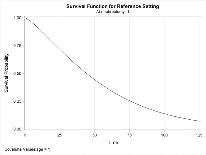
Output 63.3.4 and Output 63.3.5 show the predicted survival curves for the two strata at the reference level.
Output 63.3.4: Estimated Survival Curve at the Reference Level for Stratum 1
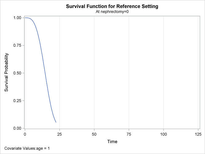
Output 63.3.5: Estimated Survival Curve at the Reference Level for Stratum 2